一、Python时间序列小波分析——实例分析

小波分析是在Fourier分析基础上发展起来的一种新的时频局部化分析方法。小波分析的基本思想是用一簇小波函数系来表示或逼近某一信号或函数。
小波分析原理涉及到傅里叶变换，并有多种小波变换，有点点小复杂。但是不会原理没关系，只要会应用并解释就可以。
在时间序列分析中，小波分析主要用于时间序列的消噪和滤波，信息量系数和分形维数的计算，突变点的检测和周期成分的识别以及多时间尺度的分析等。

小波分析通常以matlab软件为主，具体可以参考 小波系数等值线图和小波方差图绘制教学，视频教学可以参考 全网最简单的小波系数等值线图和小波方差图绘制小白教学。
matlab大多数人是不会用滴，而且安装、上手慢，不如试试Python实现小波分析。
最近在做项目中使用小波分析做时间序列分析，从零开始，学习过程还是有点痛苦，经过学习，已经初步能够解释说明输出图，特此记录一下，供大家参考。
在学习中曾经想在某宝找人做，结果要价600元，一下激发了我的征服欲，赚了自己600元，哈哈哈。
python上手简单，实现方便。PyWavelets 是一个免费的开源库，用于 Python 中的小波变换。全网对于小波分析使用python进行实例分析解释说明几乎没有，下面一步一步的介绍，给大家省600元。

pip install pycwt   #安装

PyWavelets 的主要特点是:

• 1D、2D 和 nD 正向和反向离散小波变换（DWT 和 IDWT）
• 一维、二维和 nD 多级 DWT 和 IDWT
• 一维和二维稳态小波变换（Undecimated Wavelet TransfORM）
• 一维和二维小波包分解和重建
• 一维连续小波变换
• 计算小波和缩放函数的近似值
• 超过 100 个内置小波滤波器并支持自定义小波
• 单精度和双精度计算
• 真实而复杂的计算
• 与 Matlab Wavelet Toolbox ™ 兼容的结果
  PyWavelets给出了一个例子，我感觉解释说明不清晰。

from __future__ import divisionimport numpyfrom matplotlib import pyplotimport pycwt as waveletfrom pycwt.helpers import findurl = 'Http://paos.colorado.edu/research/wavelets/wave_idl/nino3sst.txt'dat = numpy.genfromtxt(url, skip_header=19)title = 'NINO3 Sea Surface Temperature'label = 'NINO3 SST'units = 'deGC't0 = 1871.0dt = 0.25  # In yearsN = dat.sizet = numpy.arange(0, N) * dt + t0p = numpy.polyfit(t - t0, dat, 1)dat_notrend = dat - numpy.polyval(p, t - t0)std = dat_notrend.std()  # Standard deviationvar = std ** 2  # Variancedat_norm = dat_notrend / std  # Normalized datasetmother = wavelet.Morlet(6)s0 = 2 * dt  # Starting scale, in this case 2 * 0.25 years = 6 monthsdj = 1 / 12  # Twelve sub-octaves per octavesJ = 7 / dj  # Seven powers of two with dj sub-octavesalpha, _, _ = wavelet.ar1(dat)  # Lag-1 autocorrelation for red noisewave, scales, freqs, coi, fft, fftfreqs = wavelet.cwt(dat_norm, dt, dj, s0, J, mother)iwave = wavelet.icwt(wave, scales, dt, dj, mother) * stdpower = (numpy.abs(wave)) ** 2fft_power = numpy.abs(fft) ** 2period = 1 / freqspower /= scales[:, None]signif, fft_theor = wavelet.significance(1.0, dt, scales, 0, alpha,             significance_level=0.95,             wavelet=mother)sig95 = numpy.ones([1, N]) * signif[:, None]sig95 = power / sig95glbl_power = power.mean(axis=1)dof = N - scales  # Correction for padding at edgesglbl_signif, tmp = wavelet.significance(var, dt, scales, 1, alpha,            significance_level=0.95,               dof=dof,            wavelet=mother)sel = find((period >= 2) & (period < 8))Cdelta = mother.cdeltascale_avg = (scales * numpy.ones((N, 1))).transpose()scale_avg = power / scale_avg  # As in Torrence and Compo (1998) equation 24scale_avg = var * dj * dt / Cdelta * scale_avg[sel, :].sum(axis=0)scale_avg_signif, tmp = wavelet.significance(var, dt, scales, 2, alpha,                 significance_level=0.95,                 dof=[scales[sel[0]],                      scales[sel[-1]]],                 wavelet=mother)# Prepare the figurepyplot.close('all')pyplot.ioff()figprops = dict(figsize=(11, 8), dpi=72)fig = pyplot.figure(**figprops)# First sub-plot, the original time series anomaly and inverse wavelet# transform.ax = pyplot.axes([0.1, 0.75, 0.65, 0.2])ax.plot(t, iwave, '-', linewidth=1, color=[0.5, 0.5, 0.5])ax.plot(t, dat, 'k', linewidth=1.5)ax.set_title('a) {}'.format(title))ax.set_ylabel(r'{} [{}]'.format(label, units))# Second sub-plot, the normalized wavelet power spectrum and significance# level contour lines and cone of influece hatched area. Note that period# scale is logarithmic.bx = pyplot.axes([0.1, 0.37, 0.65, 0.28], sharex=ax)levels = [0.0625, 0.125, 0.25, 0.5, 1, 2, 4, 8, 16]bx.contourf(t, numpy.log2(period), numpy.log2(power), numpy.log2(levels),            extend='both', cmap=pyplot.cm.viridis)extent = [t.min(), t.max(), 0, max(period)]bx.contour(t, numpy.log2(period), sig95, [-99, 1], colors='k', linewidths=2,           extent=extent)bx.fill(numpy.concatenate([t, t[-1:] + dt, t[-1:] + dt,                           t[:1] - dt, t[:1] - dt]),        numpy.concatenate([numpy.log2(coi), [1e-9], numpy.log2(period[-1:]),                           numpy.log2(period[-1:]), [1e-9]]),        'k', alpha=0.3, hatch='x')bx.set_title('b) {} Wavelet Power Spectrum ({})'.format(label, mother.name))bx.set_ylabel('Period (years)')#Yticks = 2 ** numpy.arange(numpy.ceil(numpy.log2(period.min())),                           numpy.ceil(numpy.log2(period.max())))bx.set_yticks(numpy.log2(Yticks))bx.set_yticklabels(Yticks)# Third sub-plot, the global wavelet and Fourier power spectra and theoretical# noise spectra. Note that period scale is logarithmic.cx = pyplot.axes([0.77, 0.37, 0.2, 0.28], sharey=bx)cx.plot(glbl_signif, numpy.log2(period), 'k--')cx.plot(var * fft_theor, numpy.log2(period), '--', color='#cccccc')cx.plot(var * fft_power, numpy.log2(1./fftfreqs), '-', color='#cccccc',        linewidth=1.)cx.plot(var * glbl_power, numpy.log2(period), 'k-', linewidth=1.5)cx.set_title('c) Global Wavelet Spectrum')cx.set_xlabel(r'Power [({})^2]'.format(units))cx.set_xlim([0, glbl_power.max() + var])cx.set_ylim(numpy.log2([period.min(), period.max()]))cx.set_yticks(numpy.log2(Yticks))cx.set_yticklabels(Yticks)pyplot.setp(cx.get_yticklabels(), visible=False)# Fourth sub-plot, the scale averaged wavelet spectrum.dx = pyplot.axes([0.1, 0.07, 0.65, 0.2], sharex=ax)dx.axhline(scale_avg_signif, color='k', linestyle='--', linewidth=1.)dx.plot(t, scale_avg, 'k-', linewidth=1.5)dx.set_title('d) {}--{} year scale-averaged power'.format(2, 8))dx.set_xlabel('Time (year)')dx.set_ylabel(r'Average variance [{}]'.format(units))ax.set_xlim([t.min(), t.max()])pyplot.show()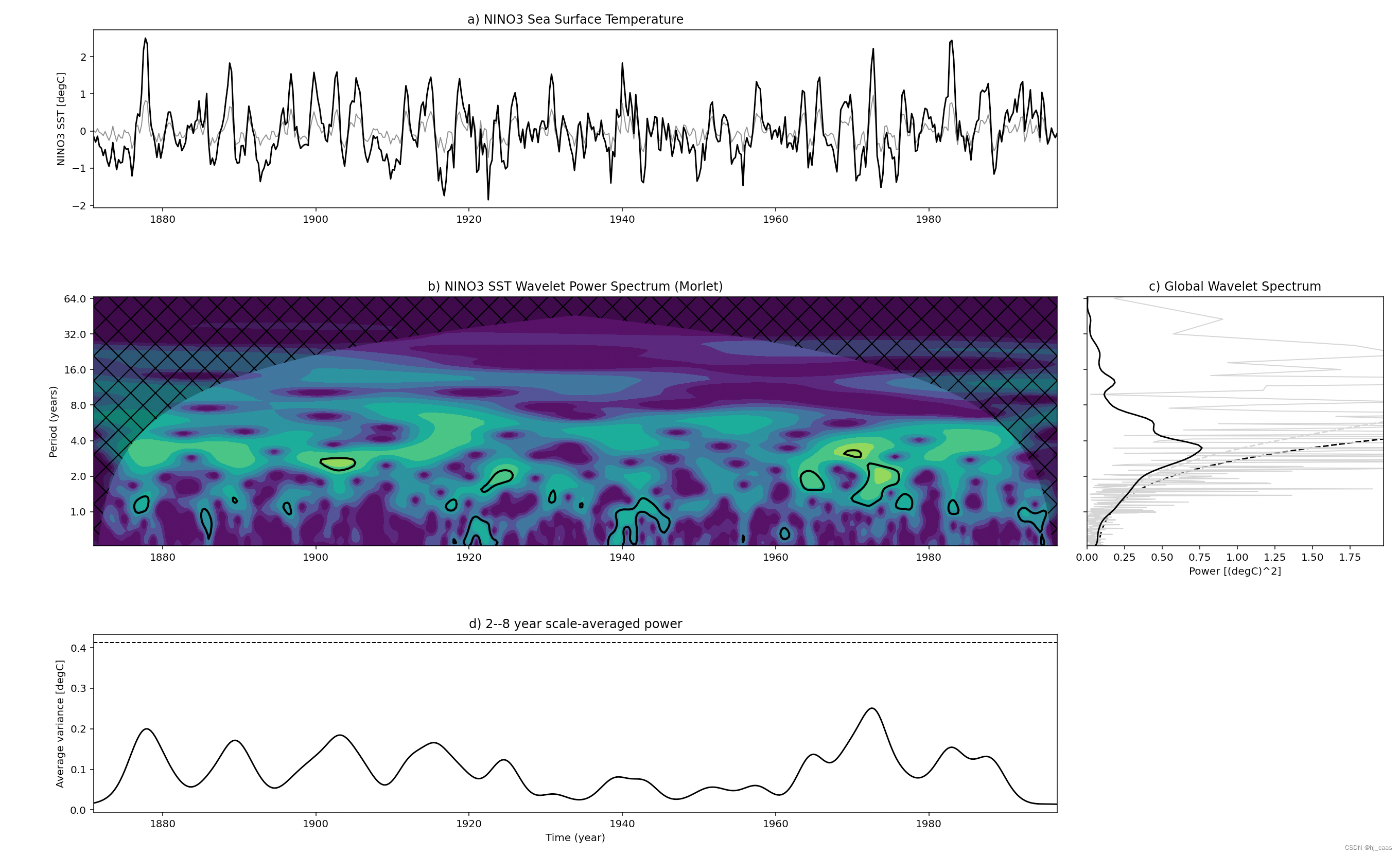

后续将以自己的数据集对输出图进行解释说明，其中输出图包括小波系数实部等值线图，小波系数方差图，小波系数模的平方图，以及主周期趋势图，分析不同时间尺度下的时间周期。

来源地址：https://blog.csdn.net/weixin_48030475/article/details/129070265