Python 官方文档:入门教程 => 点击学习
目录分类网络的常见形式分类网络介绍1、VGG16网络介绍2、MobilenetV1网络介绍3、ResNet50网络介绍a、什么是残差网络b、什么是ResNet50模型分类网络的训练1
才发现做了这么多的博客和视频,居然从来没有系统地做过分类网络,做一个科学的分类网络,对身体好。
源码下载
常见的分类网络都可以分为两部分,一部分是特征提取部分,另一部分是分类部分。

特征提取部分的功能是对输入进来的图片进行特征提取,优秀的特征可以帮助更容易区分目标,所以特征提取部分一般由各类卷积组成,卷积拥有强大的特征提取能力;
分类部分会利用特征提取部分获取到的特征进行分类,分类部分一般由全连接组成,特征提取部分获取到的特征一般是一维向量,可以直接进行全连接分类。
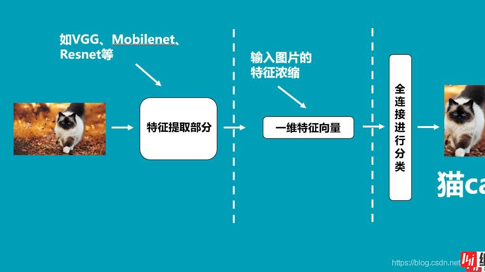
通常情况下,特征提取部分就是我们平常了解到的各种神经网络,比如VGG、Mobilenet、Resnet等等;而分类部分就是一次或者几次的全连接,最终我们会获得一个长度为num_classes的一维向量。
VGG是由Simonyan 和Zisserman在文献《Very Deep Convolutional Networks for Large Scale Image Recognition》中提出卷积神经网络模型,其名称来源于作者所在的牛津大学视觉几何组(Visual Geometry Group)的缩写。
该模型参加2014年的 ImageNet图像分类与定位挑战赛,取得了优异成绩:在分类任务上排名第二,在定位任务上排名第一。
它的结构如下图所示:

这是一个VGG16被用到烂的图,但确实很好的反应了VGG16的结构,整个VGG16由三种不同的层组成,分别是卷积层、最大池化层、全连接层。
VGG16的具体执行方式如下:
1、一张原始图片被resize到(224,224,3)。
2、conv1:进行两次[3,3]卷积网络,输出的特征层为64,输出为(224,224,64),再进行2X2最大池化,输出net为(112,112,64)。
3、conv2:进行两次[3,3]卷积网络,输出的特征层为128,输出net为(112,112,128),再进行2X2最大池化,输出net为(56,56,128)。
4、conv3:进行三次[3,3]卷积网络,输出的特征层为256,输出net为(56,56,256),再进行2X2最大池化,输出net为(28,28,256)。
5、conv4:进行三次[3,3]卷积网络,输出的特征层为512,输出net为(28,28,512),再进行2X2最大池化,输出net为(14,14,512)。
6、conv5:进行三次[3,3]卷积网络,输出的特征层为512,输出net为(14,14,512),再进行2X2最大池化,输出net为(7,7,512)。
7、对结果进行平铺。
8、进行两次神经元为4096的全连接层。
9、全连接到1000维上,用于进行分类。
最后输出的就是每个类的预测。
实现代码如下:
import warnings
from keras.models import Model
from keras.layers import Input,Activation,Dropout,Reshape,Conv2D,MaxPooling2D,Dense,Flatten
from keras import backend as K
def VGG16(input_shape=None, classes=1000):
    img_input = Input(shape=input_shape)
    # Block 1
    x = Conv2D(64, (3, 3),
                      activation='relu',
                      padding='same',
                      name='block1_conv1')(img_input)
    x = Conv2D(64, (3, 3),
                      activation='relu',
                      padding='same',
                      name='block1_conv2')(x)
    x = MaxPooling2D((2, 2), strides=(2, 2), name='block1_pool')(x)
    # Block 2
    x = Conv2D(128, (3, 3),
                      activation='relu',
                      padding='same',
                      name='block2_conv1')(x)
    x = Conv2D(128, (3, 3),
                      activation='relu',
                      padding='same',
                      name='block2_conv2')(x)
    x = MaxPooling2D((2, 2), strides=(2, 2), name='block2_pool')(x)
    # Block 3
    x = Conv2D(256, (3, 3),
                      activation='relu',
                      padding='same',
                      name='block3_conv1')(x)
    x = Conv2D(256, (3, 3),
                      activation='relu',
                      padding='same',
                      name='block3_conv2')(x)
    x = Conv2D(256, (3, 3),
                      activation='relu',
                      padding='same',
                      name='block3_conv3')(x)
    x = MaxPooling2D((2, 2), strides=(2, 2), name='block3_pool')(x)
    # Block 4
    x = Conv2D(512, (3, 3),
                      activation='relu',
                      padding='same',
                      name='block4_conv1')(x)
    x = Conv2D(512, (3, 3),
                      activation='relu',
                      padding='same',
                      name='block4_conv2')(x)
    x = Conv2D(512, (3, 3),
                      activation='relu',
                      padding='same',
                      name='block4_conv3')(x)
    x = MaxPooling2D((2, 2), strides=(2, 2), name='block4_pool')(x)
    # Block 5
    x = Conv2D(512, (3, 3),
                      activation='relu',
                      padding='same',
                      name='block5_conv1')(x)
    x = Conv2D(512, (3, 3),
                      activation='relu',
                      padding='same',
                      name='block5_conv2')(x)
    x = Conv2D(512, (3, 3),
                      activation='relu',
                      padding='same',
                      name='block5_conv3')(x)
    x = MaxPooling2D((2, 2), strides=(2, 2), name='block5_pool')(x)
    x = Flatten(name='flatten')(x)
    x = Dense(4096, activation='relu', name='fc1')(x)
    x = Dense(4096, activation='relu', name='fc2')(x)
    x = Dense(classes, activation='softmax', name='predictions')(x)
    inputs = img_input
    model = Model(inputs, x, name='vgg16')
    return model
MobilenetV1模型是Google针对手机等嵌入式设备提出的一种轻量级的深层神经网络,其使用的核心思想便是depthwise separable convolution(深度可分离卷积块)。
深度可分离卷积块由两个部分组成,分别是深度可分离卷积和1x1普通卷积,深度可分离卷积的卷积核大小一般是3x3的,便于理解的话我们可以把它当作是特征提取,1x1的普通卷积可以完成通道数的调整。
下图为深度可分离卷积块的结构示意图:

深度可分离卷积块的目的是使用更少的参数来代替普通的3x3卷积。
我们可以进行一下普通卷积和深度可分离卷积块的对比:
对于普通卷积而言,假设有一个3×3大小的卷积层,其输入通道为16、输出通道为32。具体为,32个3×3大小的卷积核会遍历16个通道中的每个数据,最后可得到所需的32个输出通道,所需参数为16×32×3×3=4608个。
对于深度可分离卷积结构块而言,假设有一个深度可分离卷积结构块,其输入通道为16、输出通道为32,其会用16个3×3大小的卷积核分别遍历16通道的数据,得到了16个特征图谱。在融合操作之前,接着用32个1×1大小的卷积核遍历这16个特征图谱,所需参数为16×3×3+16×32×1×1=656个。
可以看出来深度可分离卷积结构块可以减少模型的参数。
深度可分离卷积的代码如下:
def _depthwise_conv_block(inputs, pointwise_conv_filters, alpha,
                          depth_multiplier=1, strides=(1, 1), block_id=1):
    pointwise_conv_filters = int(pointwise_conv_filters * alpha)
    x = DepthwiseConv2D((3, 3),
                        padding='same',
                        depth_multiplier=depth_multiplier,
                        strides=strides,
                        use_bias=False,
                        name='conv_dw_%d' % block_id)(inputs)
    x = BatchNORMalization(name='conv_dw_%d_bn' % block_id)(x)
    x = Activation(relu6, name='conv_dw_%d_relu' % block_id)(x)
    x = Conv2D(pointwise_conv_filters, (1, 1),
               padding='same',
               use_bias=False,
               strides=(1, 1),
               name='conv_pw_%d' % block_id)(x)
    x = BatchNormalization(name='conv_pw_%d_bn' % block_id)(x)
    return Activation(relu6, name='conv_pw_%d_relu' % block_id)(x)
通俗地理解深度可分离卷积结构块,就是3x3的卷积核厚度只有一层,然后在输入张量上一层一层地滑动,每一次卷积完生成一个输出通道,当卷积完成后,在利用1x1的卷积调整厚度。
如下就是MobileNet的结构,其中Conv dw就是深度可分离卷积,在其之后都会接一个1x1的卷积进行通道处理,

在利用特征提取部分完成输入图片的特征提取后,我们会利用全局平均池化将特征层调整成一个特征长条,我们可以将特征长条进行全连接,获得最终的分类结果。
实现代码如下:
import warnings
from keras.models import Model
from keras.layers import DepthwiseConv2D,Input,Activation,Dropout,Reshape,BatchNormalization,GlobalAveragePooling2D,GlobalMaxPooling2D,Conv2D
from keras import backend as K
def _conv_block(inputs, filters, alpha, kernel=(3, 3), strides=(1, 1)):
    filters = int(filters * alpha)
    x = Conv2D(filters, kernel,
                      padding='same',
                      use_bias=False,
                      strides=strides,
                      name='conv1')(inputs)
    x = BatchNormalization(name='conv1_bn')(x)
    return Activation(relu6, name='conv1_relu')(x)
def _depthwise_conv_block(inputs, pointwise_conv_filters, alpha,
                          depth_multiplier=1, strides=(1, 1), block_id=1):
    pointwise_conv_filters = int(pointwise_conv_filters * alpha)
    x = DepthwiseConv2D((3, 3),
                        padding='same',
                        depth_multiplier=depth_multiplier,
                        strides=strides,
                        use_bias=False,
                        name='conv_dw_%d' % block_id)(inputs)
    x = BatchNormalization(name='conv_dw_%d_bn' % block_id)(x)
    x = Activation(relu6, name='conv_dw_%d_relu' % block_id)(x)
    x = Conv2D(pointwise_conv_filters, (1, 1),
               padding='same',
               use_bias=False,
               strides=(1, 1),
               name='conv_pw_%d' % block_id)(x)
    x = BatchNormalization(name='conv_pw_%d_bn' % block_id)(x)
    return Activation(relu6, name='conv_pw_%d_relu' % block_id)(x)
def MobileNet(input_shape=None,
              alpha=1.0,
              depth_multiplier=1,
              dropout=1e-3,
              classes=1000):
    img_input = Input(shape=input_shape)
    # 224,224,3 -> 112,112,32
    x = _conv_block(img_input, 32, alpha, strides=(2, 2))
    # 112,112,32 -> 112,112,64
    x = _depthwise_conv_block(x, 64, alpha, depth_multiplier, block_id=1)
    # 112,112,64 -> 56,56,128
    x = _depthwise_conv_block(x, 128, alpha, depth_multiplier,
                              strides=(2, 2), block_id=2)
    x = _depthwise_conv_block(x, 128, alpha, depth_multiplier, block_id=3)
    # 56,56,128 -> 28,28,256
    x = _depthwise_conv_block(x, 256, alpha, depth_multiplier,
                              strides=(2, 2), block_id=4)
    x = _depthwise_conv_block(x, 256, alpha, depth_multiplier, block_id=5)
    # 28,28,256 -> 14,14,512
    x = _depthwise_conv_block(x, 512, alpha, depth_multiplier,
                              strides=(2, 2), block_id=6)
    x = _depthwise_conv_block(x, 512, alpha, depth_multiplier, block_id=7)
    x = _depthwise_conv_block(x, 512, alpha, depth_multiplier, block_id=8)
    x = _depthwise_conv_block(x, 512, alpha, depth_multiplier, block_id=9)
    x = _depthwise_conv_block(x, 512, alpha, depth_multiplier, block_id=10)
    x = _depthwise_conv_block(x, 512, alpha, depth_multiplier, block_id=11)
    # 14,14,512 -> 7,7,1024
    x = _depthwise_conv_block(x, 1024, alpha, depth_multiplier,
                              strides=(2, 2), block_id=12)
    x = _depthwise_conv_block(x, 1024, alpha, depth_multiplier, block_id=13)
    # 7,7,1024 -> 1,1,1024
    x = GlobalAveragePooling2D()(x)
    shape = (1, 1, int(1024 * alpha))
    x = Reshape(shape, name='reshape_1')(x)
    x = Dropout(dropout, name='dropout')(x)
    x = Conv2D(classes, (1, 1),padding='same', name='conv_preds')(x)
    x = Activation('softmax', name='act_softmax')(x)
    x = Reshape((classes,), name='reshape_2')(x)
    inputs = img_input
    model = Model(inputs, x, name='mobilenet_%0.2f' % (alpha))
    return model
def relu6(x):
    return K.relu(x, max_value=6)
if __name__ == '__main__':
    model = MobileNet(input_shape=(224, 224, 3))
    model.summary()
Residual net(残差网络):
将靠前若干层的某一层数据输出直接跳过多层引入到后面数据层的输入部分。
意味着后面的特征层的内容会有一部分由其前面的某一层线性贡献。
其结构如下:

深度残差网络的设计是为了克服由于网络深度加深而产生的学习效率变低与准确率无法有效提升的问题。
ResNet50有两个基本的块,分别名为Conv Block和Identity Block,其中Conv Block输入和输出的维度是不一样的,所以不能连续串联,它的作用是改变网络的维度;Identity Block输入维度和输出维度相同,可以串联,用于加深网络的。
Conv Block的结构如下,由图可以看出,Conv Block可以分为两个部分,左边部分为主干部分,存在两次卷积、标准化、激活函数和一次卷积、标准化;
右边部分为残差边部分,存在一次卷积、标准化,由于残差边部分存在卷积,所以我们可以利用Conv Block改变输出特征层的宽高和通道数:

实现代码如下:
def conv_block(input_tensor, kernel_size, filters, stage, block, strides=(2, 2)):
    filters1, filters2, filters3 = filters
    conv_name_base = 'res' + str(stage) + block + '_branch'
    bn_name_base = 'bn' + str(stage) + block + '_branch'
    # 降维
    x = Conv2D(filters1, (1, 1), strides=strides,
               name=conv_name_base + '2a')(input_tensor)
    x = BatchNormalization(name=bn_name_base + '2a')(x)
    x = Activation('relu')(x)
    # 3x3卷积
    x = Conv2D(filters2, kernel_size, padding='same',
               name=conv_name_base + '2b')(x)
    x = BatchNormalization(name=bn_name_base + '2b')(x)
    x = Activation('relu')(x)
    # 升维
    x = Conv2D(filters3, (1, 1), name=conv_name_base + '2c')(x)
    x = BatchNormalization(name=bn_name_base + '2c')(x)
    # 残差边
    shortcut = Conv2D(filters3, (1, 1), strides=strides,
                      name=conv_name_base + '1')(input_tensor)
    shortcut = BatchNormalization(name=bn_name_base + '1')(shortcut)
    x = layers.add([x, shortcut])
    x = Activation('relu')(x)
    return x
Identity Block的结构如下,由图可以看出,Identity Block可以分为两个部分,左边部分为主干部分,存在两次卷积、标准化、激活函数和一次卷积、标准化;右边部分为残差边部分,直接与输出相接,由于残差边部分不存在卷积,所以Identity Block的输入特征层和输出特征层的shape是相同的,可用于加深网络:

实现代码如下:
def identity_block(input_tensor, kernel_size, filters, stage, block):
    filters1, filters2, filters3 = filters
    conv_name_base = 'res' + str(stage) + block + '_branch'
    bn_name_base = 'bn' + str(stage) + block + '_branch'
    # 降维
    x = Conv2D(filters1, (1, 1), name=conv_name_base + '2a')(input_tensor)
    x = BatchNormalization(name=bn_name_base + '2a')(x)
    x = Activation('relu')(x)
    # 3x3卷积
    x = Conv2D(filters2, kernel_size,padding='same', name=conv_name_base + '2b')(x)
    x = BatchNormalization(name=bn_name_base + '2b')(x)
    x = Activation('relu')(x)
    # 升维
    x = Conv2D(filters3, (1, 1), name=conv_name_base + '2c')(x)
    x = BatchNormalization(name=bn_name_base + '2c')(x)
    x = layers.add([x, input_tensor])
    x = Activation('relu')(x)
    return x
Conv Block和Identity Block都是残差网络结构。
总的网络结构如下:

实现代码如下:
from __future__ import print_function
import numpy as np
from keras import layers
from keras.layers import Input
from keras.layers import Dense,Conv2D,MaxPooling2D,ZeroPadding2D,AveragePooling2D
from keras.layers import Activation,BatchNormalization,Flatten
from keras.models import Model
def identity_block(input_tensor, kernel_size, filters, stage, block):
    filters1, filters2, filters3 = filters
    conv_name_base = 'res' + str(stage) + block + '_branch'
    bn_name_base = 'bn' + str(stage) + block + '_branch'
    # 降维
    x = Conv2D(filters1, (1, 1), name=conv_name_base + '2a')(input_tensor)
    x = BatchNormalization(name=bn_name_base + '2a')(x)
    x = Activation('relu')(x)
    # 3x3卷积
    x = Conv2D(filters2, kernel_size,padding='same', name=conv_name_base + '2b')(x)
    x = BatchNormalization(name=bn_name_base + '2b')(x)
    x = Activation('relu')(x)
    # 升维
    x = Conv2D(filters3, (1, 1), name=conv_name_base + '2c')(x)
    x = BatchNormalization(name=bn_name_base + '2c')(x)
    x = layers.add([x, input_tensor])
    x = Activation('relu')(x)
    return x
def conv_block(input_tensor, kernel_size, filters, stage, block, strides=(2, 2)):
    filters1, filters2, filters3 = filters
    conv_name_base = 'res' + str(stage) + block + '_branch'
    bn_name_base = 'bn' + str(stage) + block + '_branch'
    # 降维
    x = Conv2D(filters1, (1, 1), strides=strides,
               name=conv_name_base + '2a')(input_tensor)
    x = BatchNormalization(name=bn_name_base + '2a')(x)
    x = Activation('relu')(x)
    # 3x3卷积
    x = Conv2D(filters2, kernel_size, padding='same',
               name=conv_name_base + '2b')(x)
    x = BatchNormalization(name=bn_name_base + '2b')(x)
    x = Activation('relu')(x)
    # 升维
    x = Conv2D(filters3, (1, 1), name=conv_name_base + '2c')(x)
    x = BatchNormalization(name=bn_name_base + '2c')(x)
    # 残差边
    shortcut = Conv2D(filters3, (1, 1), strides=strides,
                      name=conv_name_base + '1')(input_tensor)
    shortcut = BatchNormalization(name=bn_name_base + '1')(shortcut)
    x = layers.add([x, shortcut])
    x = Activation('relu')(x)
    return x
def ResNet50(input_shape=[224,224,3], classes=1000):
    # 224,224,3
    img_input = Input(shape=input_shape)
    x = ZeroPadding2D((3, 3))(img_input)
    # [112,112,64]
    x = Conv2D(64, (7, 7), strides=(2, 2), name='conv1')(x)
    x = BatchNormalization(name='bn_conv1')(x)
    x = Activation('relu')(x)
    x = ZeroPadding2D((1, 1))(x)
    # [56,56,64]
    x = MaxPooling2D((3, 3), strides=(2, 2))(x)
    # [56,56,256]
    x = conv_block(x, 3, [64, 64, 256], stage=2, block='a', strides=(1, 1))
    x = identity_block(x, 3, [64, 64, 256], stage=2, block='b')
    x = identity_block(x, 3, [64, 64, 256], stage=2, block='c')
    # [28,28,512]
    x = conv_block(x, 3, [128, 128, 512], stage=3, block='a')
    x = identity_block(x, 3, [128, 128, 512], stage=3, block='b')
    x = identity_block(x, 3, [128, 128, 512], stage=3, block='c')
    x = identity_block(x, 3, [128, 128, 512], stage=3, block='d')
    # [14,14,1024]
    x = conv_block(x, 3, [256, 256, 1024], stage=4, block='a')
    x = identity_block(x, 3, [256, 256, 1024], stage=4, block='b')
    x = identity_block(x, 3, [256, 256, 1024], stage=4, block='c')
    x = identity_block(x, 3, [256, 256, 1024], stage=4, block='d')
    x = identity_block(x, 3, [256, 256, 1024], stage=4, block='e')
    x = identity_block(x, 3, [256, 256, 1024], stage=4, block='f')
    # [7,7,2048]
    x = conv_block(x, 3, [512, 512, 2048], stage=5, block='a')
    x = identity_block(x, 3, [512, 512, 2048], stage=5, block='b')
    x = identity_block(x, 3, [512, 512, 2048], stage=5, block='c')
    # 代替全连接层
    x = AveragePooling2D((7, 7), name='avg_pool')(x)
    # 进行预测
    x = Flatten()(x)
    x = Dense(classes, activation='softmax', name='fc1000')(x)
    model = Model(img_input, x, name='resnet50')
    return model
if __name__ == '__main__':
    model = ResNet50()
    model.summary()
一般而言,分类网络所使用的损失函数为交叉熵损失函数,英文名为Cross Entropy,实现公式如下。

其中:

首先前往GitHub下载对应的仓库,下载完后利用解压软件解压,之后用编程软件打开文件夹。注意打开的根目录必须正确,否则相对目录不正确的情况下,代码将无法运行。一定要注意打开后的根目录是文件存放的目录。

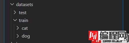
datasets文件夹下存放的是训练图片,分为两部分,train里面是训练图片,test里面是测试图片。

在训练之前需要首先准备好数据集,数据集格式为在train和test文件夹下分不同的文件夹,每个文件夹的名称为对应的类别名称,文件夹下面的图片为这个类的图片。

在准备好数据集后,需要在根目录运行txt_annotation.py生成训练所需的cls_train.txt。
运行前需要修改其中的classes,将其修改成自己需要分的类。

通过txt_annotation.py我们已经生成了cls_train.txt以及cls_test.txt,此时我们可以开始训练了。
训练的参数较多,大家可以在下载库后仔细看注释,其中最重要的部分是修改model_data文件夹下的cls_classes.txt,使其也对应自己需要分的类。

在train.py里面调整自己要选择的网络和权重后,就可以开始训练了!

以上就是Keras搭建分类网络平台VGG16 MobileNet ResNet50的详细内容,更多关于Keras搭建分类网络平台的资料请关注编程网其它相关文章!
--结束END--
本文标题: Keras搭建分类网络平台VGG16 MobileNet ResNet50
本文链接: https://www.lsjlt.com/news/117666.html(转载时请注明来源链接)
有问题或投稿请发送至: 邮箱/279061341@qq.com QQ/279061341
下载Word文档到电脑,方便收藏和打印~
2024-03-01
2024-03-01
2024-03-01
2024-02-29
2024-02-29
2024-02-29
2024-02-29
2024-02-29
2024-02-29
2024-02-29
回答
回答
回答
回答
回答
回答
回答
回答
回答
回答


官方手机版

微信公众号

商务合作


0