详解TensorFlow2实现线性回归

2024-04-02 19:04:59 232人浏览安东尼

Python 官方文档：入门教程 => 点击学习

摘要

目录概述MSE线性回归公式梯度下降线性回归实现计算 MSE梯度下降迭代训练主函数完整代码概述线性回归 (Linear Regression) 是利用回归分析来确定两种或两种以上变量

概述

线性回归 (Linear Regression) 是利用回归分析来确定两种或两种以上变量间相互依赖的定量关系.

在这里插入图片描述

对线性回归还不是很了解的同学可以看一下这篇文章:

python深度总结线性回归

MSE

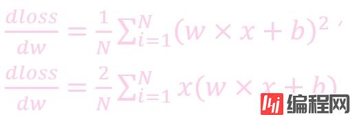
均方误差 (Mean Square Error): 是用来描述连续误差的一种方法. 公式:

在这里插入图片描述

y_predict: 我们预测的值y_real: 真实值

线性回归

公式

在这里插入图片描述

w: weight, 权重系数

b: bias, 偏置顶

x: 特征值

y: 预测值

梯度下降

梯度下降 (Gradient Descent) 是一种优化算法. 参数会沿着梯度相反的方向前进, 以实现损失函数 (loss function) 的最小化.

在这里插入图片描述

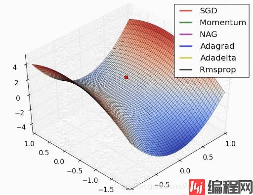
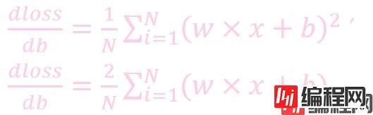
计算公式:

在这里插入图片描述

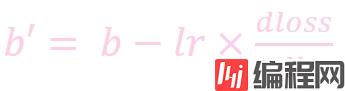
w: weight, 权重参数

w': 更新后的 weight

lr : learning rate, 学习率

dloss/dw: 损失函数对 w 求导

在这里插入图片描述

w: weight, 权重参数

w': 更新后的 weight

lr : learning rate, 学习率

dloss/dw: 损失函数对 b 求导

线性回归实现

计算 MSE


def calculate_MSE(w, b, points):
    """
    计算误差MSE
    :param w: weight, 权重
    :param b: bias, 偏置顶
    :param points: 数据
    :return: 返回MSE (Mean Square Error)
    """

    total_error = 0  # 存放总误差, 初始化为0

    # 遍历数据
    for i in range(len(points)):
        # 取出x, y
        x = points.iloc[i, 0]  # 第一列
        y = points.iloc[i, 1]  # 第二列

        # 计算MSE
        total_error += (y - (w * x + b)) ** 2  # 计总误差
        MSE = total_error / len(points)  # 计算平均误差

    # 返回MSE
    return MSE

梯度下降


def step_gradient(index, w_current, b_current, points, learning_rate=0.0001):
    """
    计算梯度下降, 跟新权重
    :param index: 现行迭代编号
    :param w_current: weight, 权重
    :param b_current: bias, 偏置顶
    :param points: 数据
    :param learning_rate: lr, 学习率 (默认值: 0.0001)
    :return: 返回跟新过后的参数数组
    """

    b_gradient = 0  # b的导, 初始化为0
    w_gradient = 0  # w的导, 初始化为0
    N = len(points)  # 数据长度

    # 遍历数据
    for i in range(len(points)):
        # 取出x, y
        x = points.iloc[i, 0]  # 第一列
        y = points.iloc[i, 1]  # 第二列

        # 计算w的导, w的导 = 2x(wx+b-y)
        w_gradient += (2 / N) * x * ((w_current * x + b_current) - y)

        # 计算b的导, b的导 = 2(wx+b-y)
        b_gradient += (2 / N) * ((w_current * x + b_current) - y)

    # 跟新w和b
    w_new = w_current - (learning_rate * w_gradient)  # 下降导数*学习率
    b_new = b_current - (learning_rate * b_gradient)  # 下降导数*学习率

    # 每迭代10次, 调试输出
    if index % 10 == 0:
        print("This is the {}th iterations w = {}, b = {}, error = {}"
              .fORMat(index, w_new, b_new,
                      calculate_MSE(w_new, b_new, points)))

    # 返回更新后的权重和偏置顶
    return [w_new, b_new]

迭代训练


def runner(w_start, b_start, points, learning_rate, num_iterations):
    """
    迭代训练
    :param w_start: 初始weight
    :param b_start: 初始bias
    :param points: 数据
    :param learning_rate: 学习率
    :param num_iterations: 迭代次数
    :return: 训练好的权重和偏执顶
    """

    # 定义w_end, b_end, 存放返回权重
    w_end = w_start
    b_end = b_start

    # 更新权重
    for i in range(1, num_iterations + 1):
        w_end, b_end = step_gradient(i, w_end, b_end, points, learning_rate)

    # 返回训练好的b, w
    return [w_end, b_end]

主函数


def run():
    """
    主函数
    :return: 无返回值
    """

    # 读取数据
    data = pd.read_csv("data.csv")  

    # 定义超参数
    learning_rate = 0.00001  # 学习率
    w_initial = 0  # 权重初始化
    b_initial = 0  # 偏置顶初始化
    w_end = 0  # 存放返回结果
    b_end = 0  # 存放返回结果
    num_interations = 200  # 迭代次数

    # 调试输出初始误差
    print("Starting gradient descent at w = {}, b = {}, error = {}"
          .format(w_initial, b_initial, calculate_MSE(w_initial, b_initial, data)))
    print("Running...")

    # 得到训练好的值
    w_end, b_end = runner(w_initial, b_initial, data, learning_rate, num_interations, )

    # 调试输出训练后的误差
    print("\nAfter {} iterations w = {}, b = {}, error = {}"
          .format(num_interations, w_end, b_end, calculate_MSE(w_end, b_end, data)))

完整代码


import pandas as pd
import Tensorflow as tf


def run():
    """
    主函数
    :return: 无返回值
    """

    # 读取数据
    data = pd.read_csv("data.csv")

    # 定义超参数
    learning_rate = 0.00001  # 学习率
    w_initial = 0  # 权重初始化
    b_initial = 0  # 偏置顶初始化
    w_end = 0  # 存放返回结果
    b_end = 0  # 存放返回结果
    num_interations = 200  # 迭代次数

    # 调试输出初始误差
    print("Starting gradient descent at w = {}, b = {}, error = {}"
          .format(w_initial, b_initial, calculate_MSE(w_initial, b_initial, data)))
    print("Running...")

    # 得到训练好的值
    w_end, b_end = runner(w_initial, b_initial, data, learning_rate, num_interations, )

    # 调试输出训练后的误差
    print("\nAfter {} iterations w = {}, b = {}, error = {}"
          .format(num_interations, w_end, b_end, calculate_MSE(w_end, b_end, data)))


def calculate_MSE(w, b, points):
    """
    计算误差MSE
    :param w: weight, 权重
    :param b: bias, 偏置顶
    :param points: 数据
    :return: 返回MSE (Mean Square Error)
    """

    total_error = 0  # 存放总误差, 初始化为0

    # 遍历数据
    for i in range(len(points)):
        # 取出x, y
        x = points.iloc[i, 0]  # 第一列
        y = points.iloc[i, 1]  # 第二列

        # 计算MSE
        total_error += (y - (w * x + b)) ** 2  # 计总误差
        MSE = total_error / len(points)  # 计算平均误差

    # 返回MSE
    return MSE


def step_gradient(index, w_current, b_current, points, learning_rate=0.0001):
    """
    计算梯度下降, 跟新权重
    :param index: 现行迭代编号
    :param w_current: weight, 权重
    :param b_current: bias, 偏置顶
    :param points: 数据
    :param learning_rate: lr, 学习率 (默认值: 0.0001)
    :return: 返回跟新过后的参数数组
    """

    b_gradient = 0  # b的导, 初始化为0
    w_gradient = 0  # w的导, 初始化为0
    N = len(points)  # 数据长度

    # 遍历数据
    for i in range(len(points)):
        # 取出x, y
        x = points.iloc[i, 0]  # 第一列
        y = points.iloc[i, 1]  # 第二列

        # 计算w的导, w的导 = 2x(wx+b-y)
        w_gradient += (2 / N) * x * ((w_current * x + b_current) - y)

        # 计算b的导, b的导 = 2(wx+b-y)
        b_gradient += (2 / N) * ((w_current * x + b_current) - y)

    # 跟新w和b
    w_new = w_current - (learning_rate * w_gradient)  # 下降导数*学习率
    b_new = b_current - (learning_rate * b_gradient)  # 下降导数*学习率

    # 每迭代10次, 调试输出
    if index % 10 == 0:
        print("This is the {}th iterations w = {}, b = {}, error = {}"
              .format(index, w_new, b_new,
                      calculate_MSE(w_new, b_new, points)))

    # 返回更新后的权重和偏置顶
    return [w_new, b_new]


def runner(w_start, b_start, points, learning_rate, num_iterations):
    """
    迭代训练
    :param w_start: 初始weight
    :param b_start: 初始bias
    :param points: 数据
    :param learning_rate: 学习率
    :param num_iterations: 迭代次数
    :return: 训练好的权重和偏执顶
    """

    # 定义w_end, b_end, 存放返回权重
    w_end = w_start
    b_end = b_start

    # 更新权重
    for i in range(1, num_iterations + 1):
        w_end, b_end = step_gradient(i, w_end, b_end, points, learning_rate)

    # 返回训练好的b, w
    return [w_end, b_end]


if __name__ == "__main__":  # 判断是否为直接运行
    # 执行主函数
    run()

输出结果:

Starting gradient descent at w = 0, b = 0, error = 5611.166153823905
Running...
This is the 10th iterations w = 0.5954939346814911, b = 0.011748797759247776, error = 2077.4540105037636
This is the 20th iterations w = 0.9515563561471605, b = 0.018802975867006404, error = 814.0851271130122
This is the 30th iterations w = 1.1644557718428263, b = 0.023050105300353223, error = 362.4068500146176
This is the 40th iterations w = 1.291753898278705, b = 0.02561881917471017, error = 200.92329896151622
This is the 50th iterations w = 1.3678685455519075, b = 0.027183959773995233, error = 143.18984477036037
This is the 60th iterations w = 1.4133791147591803, b = 0.02814903475888354, error = 122.54901023376003
This is the 70th iterations w = 1.4405906232245687, b = 0.028755312994862656, error = 115.16948797045545
This is the 80th iterations w = 1.4568605956220553, b = 0.029147056093611835, error = 112.53113537539161
This is the 90th iterations w = 1.4665883081088924, b = 0.029410522232548166, error = 111.58784050644537
This is the 100th iterations w = 1.4724042147529013, b = 0.029597287663210802, error = 111.25056079777497
This is the 110th iterations w = 1.475881139890538, b = 0.029738191313600983, error = 111.12994295811941
This is the 120th iterations w = 1.477959520545057, b = 0.02985167266801462, error = 111.08678583026905
This is the 130th iterations w = 1.479201671130221, b = 0.029948757225817496, error = 111.07132237076124
This is the 140th iterations w = 1.4799438156483897, b = 0.03003603745100295, error = 111.06575992136905
This is the 150th iterations w = 1.480386992125614, b = 0.030117455167888288, error = 111.06373727064113
This is the 160th iterations w = 1.4806514069946144, b = 0.030195367306897165, error = 111.0629801653088
This is the 170th iterations w = 1.4808089351476725, b = 0.030271183144693698, error = 111.06267551686379
This is the 180th iterations w = 1.4809025526554018, b = 0.030345745328433527, error = 111.0625326308038
This is the 190th iterations w = 1.4809579561496398, b = 0.030419557701150367, error = 111.0624475783524
This is the 200th iterations w = 1.480990510387525, b = 0.030492921525124016, error = 111.06238320300855
This is the 210th iterations w = 1.4810094024003952, b = 0.030566016933760057, error = 111.06232622062124
This is the 220th iterations w = 1.4810201253791957, b = 0.030638951634017437, error = 111.0622718818556
This is the 230th iterations w = 1.4810259638611891, b = 0.030711790026994222, error = 111.06221848873447
This is the 240th iterations w = 1.481028881765914, b = 0.030784570619965538, error = 111.06216543419914
This is the 250th iterations w = 1.4810300533774932, b = 0.030857316437543122, error = 111.06211250121454
This is the 260th iterations w = 1.4810301808342632, b = 0.03093004124680784, error = 111.06205961218657
This is the 270th iterations w = 1.4810296839649824, b = 0.031002753279495907, error = 111.06200673937376
This is the 280th iterations w = 1.4810288137973704, b = 0.031075457457601333, error = 111.06195387285815
This is the 290th iterations w = 1.48102772042814, b = 0.031148156724127858, error = 111.06190100909376
This is the 300th iterations w = 1.4810264936044433, b = 0.03122085283878386, error = 111.06184814681296
This is the 310th iterations w = 1.4810251869886903, b = 0.0312935468537513, error = 111.06179528556238
This is the 320th iterations w = 1.4810238326671836, b = 0.031366239398161695, error = 111.0617424251801
This is the 330th iterations w = 1.4810224498252484, b = 0.031438930848192506, error = 111.06168956560795
This is the 340th iterations w = 1.481021049934344, b = 0.03151162142877266, error = 111.06163670682551
This is the 350th iterations w = 1.4810196398535866, b = 0.03158431127439525, error = 111.06158384882504
This is the 360th iterations w = 1.4810182236842395, b = 0.03165700046547913, error = 111.0615309916041
This is the 370th iterations w = 1.4810168038785667, b = 0.031729689050110664, error = 111.06147813516172
This is the 380th iterations w = 1.4810153819028469, b = 0.03180237705704362, error = 111.06142527949757
This is the 390th iterations w = 1.48101395863381, b = 0.03187506450347233, error = 111.06137242461139
This is the 400th iterations w = 1.48101253459568, b = 0.03194775139967933, error = 111.06131957050317
This is the 410th iterations w = 1.4810111101019028, b = 0.03202043775181446, error = 111.06126671717288
This is the 420th iterations w = 1.4810096853398989, b = 0.032093123563556446, error = 111.06121386462064
This is the 430th iterations w = 1.4810082604217312, b = 0.032165808837106485, error = 111.06116101284626
This is the 440th iterations w = 1.481006835414406, b = 0.03223849357378233, error = 111.06110816184975
This is the 450th iterations w = 1.4810054103579875, b = 0.03231117777437349, error = 111.06105531163115
This is the 460th iterations w = 1.4810039852764323, b = 0.0323838614393536, error = 111.06100246219052
This is the 470th iterations w = 1.4810025601840635, b = 0.032456544569007456, error = 111.0609496135277
This is the 480th iterations w = 1.4810011350894463, b = 0.03252922716350693, error = 111.06089676564281
This is the 490th iterations w = 1.4809997099977015, b = 0.032601909222956374, error = 111.06084391853577
This is the 500th iterations w = 1.4809982849118903, b = 0.032674590747419754, error = 111.0607910722065

After 500 iterations w = 1.4809982849118903, b = 0.032674590747419754, error = 111.0607910722065