Python&Matla实现模拟退火法的示例代码

#===========1导包================
import matplotlib.pyplot as plt
import pandas as pd
from sko.SA import SA
 
#============2定义问题===============
fun = lambda x: x[0] ** 2 + (x[1] - 0.05) ** 2 + x[2] ** 2
 
#=========3运行模拟退火算法===========
sa = SA(func=fun, x0=[1, 1, 1], T_max=1, T_min=1e-9, L=300, max_stay_counter=150)
best_x, best_y = sa.run()
print('best_x:', best_x, 'best_y', best_y)
 
#=======4画出结果=======
plt.plot(pd.DataFrame(sa.best_y_history).cummin(axis=0))
plt.show()
 
 
 
 
#scikit-opt 还提供了三种模拟退火流派: Fast, Boltzmann, Cauchy.
 
#===========1.1 Fast Simulated Annealing=====================
from sko.SA import SAFast
 
sa_fast = SAFast(func=demo_func, x0=[1, 1, 1], T_max=1, T_min=1e-9, q=0.99, L=300, max_stay_counter=150)
sa_fast.run()
print('Fast Simulated Annealing: best_x is ', sa_fast.best_x, 'best_y is ', sa_fast.best_y)
 
#===========1.2 Fast Simulated Annealing with bounds=====================
from sko.SA import SAFast
 
sa_fast = SAFast(func=demo_func, x0=[1, 1, 1], T_max=1, T_min=1e-9, q=0.99, L=300, max_stay_counter=150,
                 lb=[-1, 1, -1], ub=[2, 3, 4])
sa_fast.run()
print('Fast Simulated Annealing with bounds: best_x is ', sa_fast.best_x, 'best_y is ', sa_fast.best_y)
 
#===========2.1 Boltzmann Simulated Annealing====================
from sko.SA import SABoltzmann
 
sa_boltzmann = SABoltzmann(func=demo_func, x0=[1, 1, 1], T_max=1, T_min=1e-9, q=0.99, L=300, max_stay_counter=150)
sa_boltzmann.run()
print('Boltzmann Simulated Annealing: best_x is ', sa_boltzmann.best_x, 'best_y is ', sa_fast.best_y)
 
#===========2.2 Boltzmann Simulated Annealing with bounds====================
from sko.SA import SABoltzmann
 
sa_boltzmann = SABoltzmann(func=demo_func, x0=[1, 1, 1], T_max=1, T_min=1e-9, q=0.99, L=300, max_stay_counter=150,
                           lb=-1, ub=[2, 3, 4])
sa_boltzmann.run()
print('Boltzmann Simulated Annealing with bounds: best_x is ', sa_boltzmann.best_x, 'best_y is ', sa_fast.best_y)
 
#==================3.1 Cauchy Simulated Annealing==================
from sko.SA import SACauchy
 
sa_cauchy = SACauchy(func=demo_func, x0=[1, 1, 1], T_max=1, T_min=1e-9, q=0.99, L=300, max_stay_counter=150)
sa_cauchy.run()
print('Cauchy Simulated Annealing: best_x is ', sa_cauchy.best_x, 'best_y is ', sa_cauchy.best_y)
 
#==================3.2 Cauchy Simulated Annealing with bounds==================
from sko.SA import SACauchy
 
sa_cauchy = SACauchy(func=demo_func, x0=[1, 1, 1], T_max=1, T_min=1e-9, q=0.99, L=300, max_stay_counter=150,
                     lb=[-1, 1, -1], ub=[2, 3, 4])
sa_cauchy.run()
print('Cauchy Simulated Annealing with bounds: best_x is ', sa_cauchy.best_x, 'best_y is ', sa_cauchy.best_y)

clear
clc
T=1000; %初始化温度值
T_min=1; %设置温度下界
alpha=0.99; %温度的下降率
num=1000; %颗粒总数
n=2; %自变量个数
sub=[-5,-5]; %自变量下限
up=[5,5]; %自变量上限
tu
for i=1:num
for j=1:n
x(i,j)=(up(j)-sub(j))*rand+sub(j);
    end
    fx(i,1)=fun(x(i,1),x(i,2));
end
 
%以最小化为例
[bestf,a]=min(fx);
bestx=x(a,:);
trace(1)=bestf;
while(T>T_min)
for i=1:num
for j=1:n
            xx(i,j)=(up(j)-sub(j))*rand+sub(j);
        end
        ff(i,1)=fun(xx(i,1),xx(i,2));
        delta=ff(i,1)-fx(i,1);
if delta<0
            fx(i,1)=ff(i,1);
x(i,:)=xx(i,:);
else
            P=exp(-delta/T);
if P>rand
                fx(i,1)=ff(i,1);
x(i,:)=xx(i,:);
            end
        end  
    end
if min(fx)<bestf
        [bestf,a]=min(fx);
        bestx=x(a,:);
    end
    trace=[trace;bestf];
    T=T*alpha;
end
disp('最优解为：')
disp(bestx)
disp('最优值为：')
disp(bestf)
hold on
plot3(bestx(1),bestx(2),bestf,'ro','LineWidth',5)
figure
plot(trace)
xlabel('迭代次数')
ylabel('函数值')
title('模拟退火算法')
legend('最优值')

function z=fun(x,y)
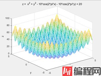
z = x.^2 + y.^2 - 10*cos(2*pi*x) - 10*cos(2*pi*y) + 20;

function tu
[x,y] = meshgrid(-5:0.1:5,-5:0.1:5);
z = x.^2 + y.^2 - 10*cos(2*pi*x) - 10*cos(2*pi*y) + 20;
figure
mesh(x,y,z)%建一个网格图，该网格图为三维曲面，有实色边颜色，无面颜色
hold on
xlabel('x')
ylabel('y')
zlabel('z')
title('z =  x^2 + y^2 - 10*cos(2*pi*x) - 10*cos(2*pi*y) + 20')

clear
clc
num=689000; %颗粒总数
n=2; %自变量个数
sub=[-5,-5]; %自变量下限
up=[5,5]; %自变量上限
tu
x=zeros(num,n);
fx=zeros(num,1);
for i=1:num
for j=1:n
x(i,j)=(up(j)-sub(j))*rand+sub(j);
    end
    fx(i,1)=fun(x(i,1),x(i,2));
end
 
[bestf,a]=min(fx);
bestx=x(a,:);
 
disp('最优解为：')
disp(bestx)
disp('最优值为：')
disp(bestf)
hold on
plot3(bestx(1),bestx(2),bestf,'ro','LineWidth',5)