Python 官方文档:入门教程 => 点击学习
目录 前言0、安装一、什么是优化问题?1-1、优化问题介绍1-2、举例1-2-1、导入所需要的库1-2-2、声明求解器1-2-3、创建变量1-2-4、定义约束条件1-2-5、定义目标函数1-2
Python -m pip install --user ortools -i https://mirror.baidu.com/pypi/simplepython -c "import ortools; print(ortools.__version__)"目标:从大量可能的解决方案中找到某个问题的最佳解决方案。
优化问题具备的元素:
1、目标,比如说最小化成本。
2、限制条件,对相关变量进行限制。
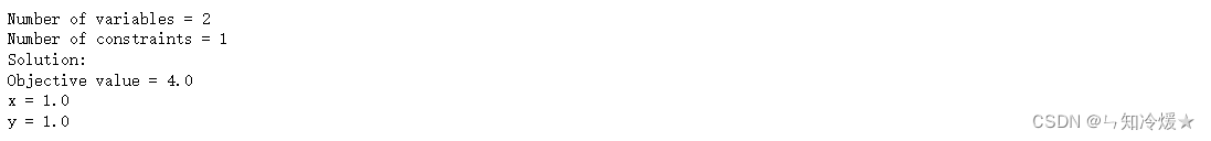
线性优化问题举例: 最大化函数3x+y,约束条件
1、 0 ≤ x ≤ 1
2、 0 ≤ y ≤ 2
3、 x + y ≤ 2
from ortools.linear_solver import pywraplpfrom ortools.init import pywrapinit# Create the linear solver with the GLOP backend.# GLOP指的是使用OR-TOOLS线性求解器solver = pywraplp.Solver.CreateSolver('GLOP')if not solver: return# Create the variables x and y.x = solver.NumVar(0, 1, 'x')y = solver.NumVar(0, 2, 'y')print('Number of variables =', solver.NumVariables())# Create a linear constraint, 0 <= x + y <= 2.ct = solver.Constraint(0, 2, 'ct')# SetCoefficient 方法用于在该限制条件的表达式中设置 x 和 y 的系数。ct.SetCoefficient(x, 1)ct.SetCoefficient(y, 1)print('Number of constraints =', solver.NumConstraints())# Create the objective function, 3 * x + y.objective = solver.Objective()objective.SetCoefficient(x, 3)objective.SetCoefficient(y, 1)# 目标函数最大化。即SetMaximization 方法将其声明为最大化问题。objective.SetMaximization()solver.Solve()print('Solution:')print('Objective value =', objective.Value())print('x =', x.solution_value())print('y =', y.solution_value())结果:
完整代码如下所示:
from ortools.linear_solver import pywraplpfrom ortools.init import pywrapinitdef main(): # Create the linear solver with the GLOP backend. solver = pywraplp.Solver.CreateSolver('GLOP') if not solver: return # Create the variables x and y. x = solver.NumVar(0, 1, 'x') y = solver.NumVar(0, 2, 'y') print('Number of variables =', solver.NumVariables()) # Create a linear constraint, 0 <= x + y <= 2. ct = solver.Constraint(0, 2, 'ct') ct.SetCoefficient(x, 1) ct.SetCoefficient(y, 1) print('Number of constraints =', solver.NumConstraints()) # Create the objective function, 3 * x + y. objective = solver.Objective() objective.SetCoefficient(x, 3) objective.SetCoefficient(y, 1) objective.SetMaximization() solver.Solve() print('Solution:') print('Objective value =', objective.Value()) print('x =', x.solution_value()) print('y =', y.solution_value())if __name__ == '__main__': pywrapinit.CppBridge.InitLogging('basic_example.py') cpp_flags = pywrapinit.CppFlags() cpp_flags.logtostderr = True cpp_flags.log_prefix = False pywrapinit.CppBridge.SetFlags(cpp_flags) main()from ortools.linear_solver import pywraplpsolver = pywraplp.Solver.CreateSolver('GLOP')# 创建x、y两个变量,范围为0——正无穷。x = solver.NumVar(0, solver.infinity(), 'x')y = solver.NumVar(0, solver.infinity(), 'y')print('Number of variables =', solver.NumVariables())# Constraint 0: x + 2y <= 14.solver.Add(x + 2 * y <= 14.0)# Constraint 1: 3x - y >= 0.solver.Add(3 * x - y >= 0.0)# Constraint 2: x - y <= 2.solver.Add(x - y <= 2.0)print('Number of constraints =', solver.NumConstraints())# Objective function: 3x + 4y.solver.Maximize(3 * x + 4 * y)# 调用求解器并输出结果status = solver.Solve()# 显示解决方案if status == pywraplp.Solver.OPTIMAL: print('Solution:') # 输出目标值以及x和y的对应值 print('Objective value =', solver.Objective().Value()) print('x =', x.solution_value()) print('y =', y.solution_value())else: print('The problem does not have an optimal solution.')# 输出花费时间以及迭代次数。print('\nAdvanced usage:')print('Problem solved in %f milliseconds' % solver.wall_time())print('Problem solved in %d iterations' % solver.iterations())输出结果: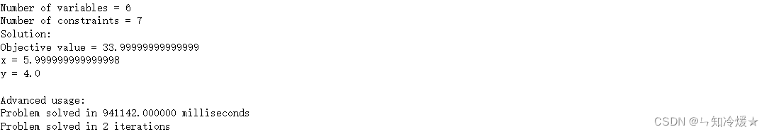
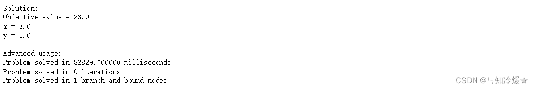
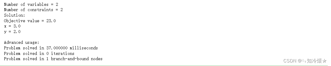
from ortools.linear_solver import pywraplpsolver = pywraplp.Solver.CreateSolver('SCIP')if solver: passelse: print('求解器不可用')infinity = solver.infinity()x = solver.IntVar(0.0, infinity, 'x')y = solver.IntVar(0.0, infinity, 'y')print('Number of variables =', solver.NumVariables())# x + 7 * y <= 17.5.solver.Add(x + 7 * y <= 17.5)# x <= 3.5.solver.Add(x <= 3.5)print('Number of constraints =', solver.NumConstraints())# Maximize x + 10 * y.solver.Maximize(x + 10 * y)status = solver.Solve()if status == pywraplp.Solver.OPTIMAL: print('Solution:') print('Objective value =', solver.Objective().Value()) print('x =', x.solution_value()) print('y =', y.solution_value())else: print('The problem does not have an optimal solution.')print('\nAdvanced usage:')print('Problem solved in %f milliseconds' % solver.wall_time())print('Problem solved in %d iterations' % solver.iterations())print('Problem solved in %d branch-and-bound nodes' % solver.nodes())输出结果:
from ortools.sat.python import cp_modeldef main(): """Minimal CP-SAT example to showcase calling the solver.""" model = cp_model.CpModel() # 取三个数中的一个最大值作为上限,这里还不是很理解啥意思。 var_upper_bound = max(50, 45, 37) # 创建变量。 x = model.NewIntVar(0, var_upper_bound, 'x') y = model.NewIntVar(0, var_upper_bound, 'y') z = model.NewIntVar(0, var_upper_bound, 'z')# 添加约束条件 model.Add(2 * x + 7 * y + 3 * z <= 50) model.Add(3 * x - 5 * y + 7 * z <= 45) model.Add(5 * x + 2 * y - 6 * z <= 37)# 添加目标函数,最小化目标函数。 model.Maximize(2 * x + 2 * y + 3 * z)# solver = cp_model.CpSolver() status = solver.Solve(model) if status == cp_model.OPTIMAL or status == cp_model.FEASIBLE: print(f'Maximum of objective function: {solver.ObjectiveValue()}\n') print(f'x = {solver.Value(x)}') print(f'y = {solver.Value(y)}') print(f'z = {solver.Value(z)}') else: print('No solution found.') print('\nStatistics') print(f' status : {solver.StatusName(status)}') print(f' conflicts: {solver.NumConflicts()}') print(f' branches : {solver.NumBranches()}') print(f' wall time: {solver.WallTime()} s') # [END statistics]if __name__ == '__main__': main()输出结果:
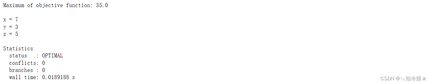
注意:为了提高计算速度,CP-SAT 求解器可以处理整数。这意味着,您只能使用整数来定义优化问题。 如果您开始遇到约束条件为非整数字词的问题,则需要先将这些约束条件乘以足够大的整数,以便所有字词都是整数。
from ortools.sat.python import cp_modeldef SolveWithTimeLimitSampleSat(): """Minimal CP-SAT example to showcase calling the solver.""" # Creates the model. model = cp_model.CpModel() # Creates the variables. # 创建变量 num_vals = 3 x = model.NewIntVar(0, num_vals - 1, 'x') y = model.NewIntVar(0, num_vals - 1, 'y') z = model.NewIntVar(0, num_vals - 1, 'z') # 添加约束条件 # Adds an all-different constraint. model.Add(x != y) # Creates a solver and solves the model. solver = cp_model.CpSolver() # 设置求解时间 # Sets a time limit of 10 seconds. solver.parameters.max_time_in_seconds = 10.0 status = solver.Solve(model) if status == cp_model.OPTIMAL: print('x = %i' % solver.Value(x)) print('y = %i' % solver.Value(y)) print('z = %i' % solver.Value(z))SolveWithTimeLimitSampleSat()# [END program]输出结果: 这里只是输出了其中一个解决方案,当然方案还有很多种。

概念: 旅行推销员问题(Travelling Salesman Problem,TSP),即给定城市列表和每对城市之间的距离,访问每个城市一次并且返回原点城市的最短路线是什么?旅行推销员问题和车辆配送问题都是TSP的概述。注意:任何TSP算法的最坏情况运行时间都可能随着城市数量的增多而超多项式增加。
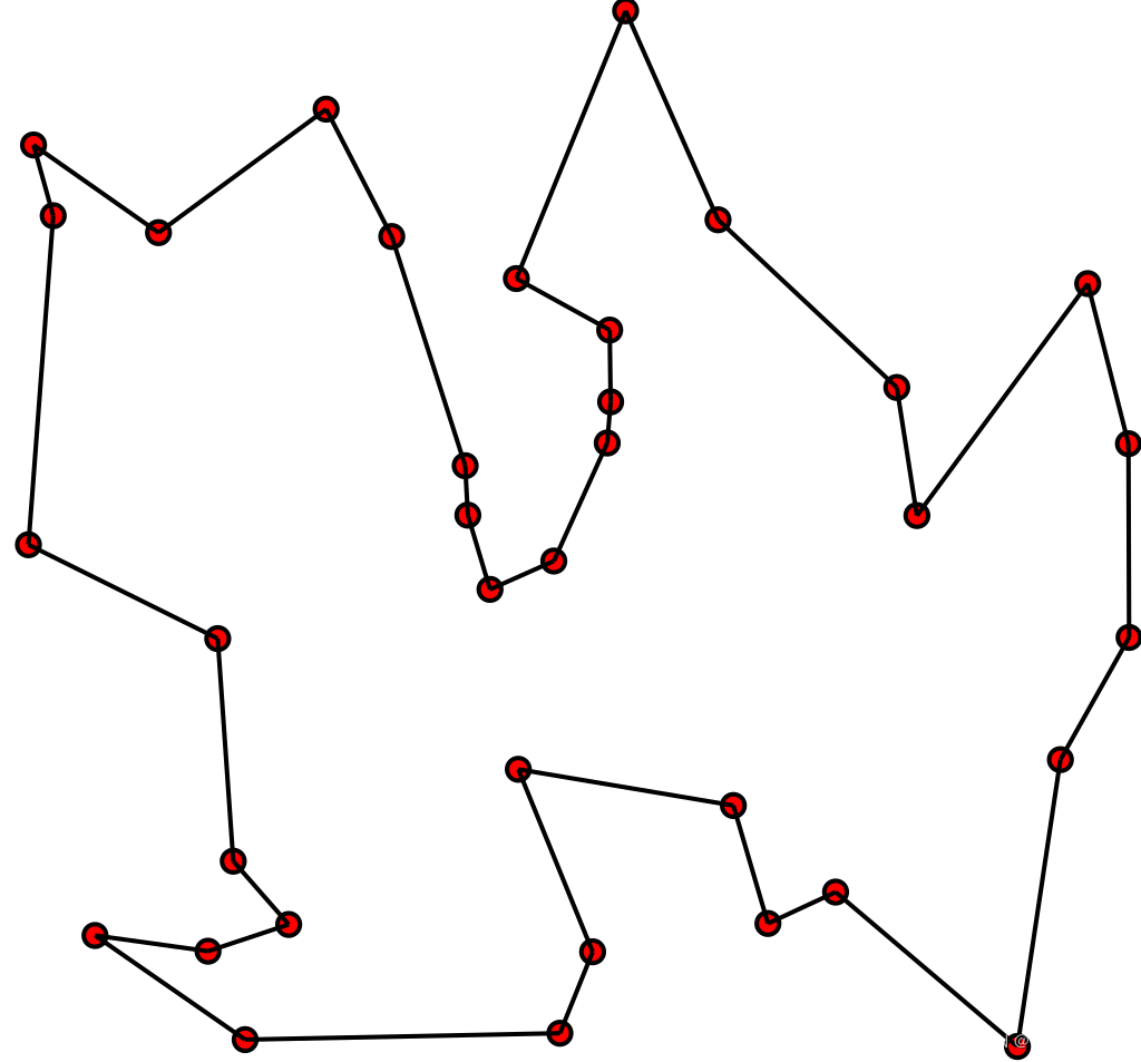
作为图形问题:TSP 可以建模为无向加权图,这样城市是图的顶点,路径是图的边,路径的距离是边的权重。这是一个最小化问题,在彼此的顶点访问过一次后,在指定的顶点开始和结束。通常,模型是一个完整的图形(即,每对顶点都由一条边连接)。如果两个城市之间不存在路径,则添加足够长的边将完成图形,而不会影响最佳游览。
MPSolver接口: 用于解决线性规划和混合整数规划问题。具体包含Glop、SCIP、CP-SAT。(这里是具体介绍这个接口的专题,有些案例可能会与上边的案例重复。)
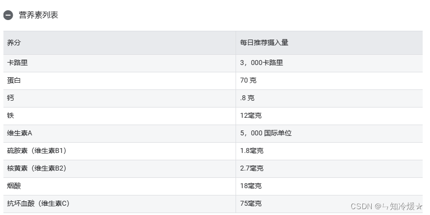
Stigler 饮食问题:如何吃的营养又花钱少。
商品清单: 这里只列出部分商品清单,详细清单请见OR-TOOLS官网。
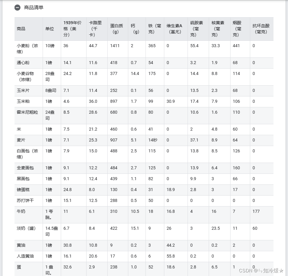
最低营养需求以及各种食物的营养数据表
# Nutrient minimums.nutrients = [ ['Calories (kcal)', 3], ['Protein (g)', 70], ['Calcium (g)', 0.8], ['Iron (mg)', 12], ['Vitamin A (KIU)', 5], ['Vitamin B1 (mg)', 1.8], ['Vitamin B2 (mg)', 2.7], ['Niacin (mg)', 18], ['Vitamin C (mg)', 75],]# Commodity, Unit, 1939 price (cents), Calories (kcal), Protein (g),# Calcium (g), Iron (mg), Vitamin A (KIU), Vitamin B1 (mg), Vitamin B2 (mg),# Niacin (mg), Vitamin C (mg)data = [ [ 'Wheat Flour (Enriched)', '10 lb.', 36, 44.7, 1411, 2, 365, 0, 55.4, 33.3, 441, 0 ], ['Macaroni', '1 lb.', 14.1, 11.6, 418, 0.7, 54, 0, 3.2, 1.9, 68, 0], [ 'Wheat Cereal (Enriched)', '28 oz.', 24.2, 11.8, 377, 14.4, 175, 0, 14.4, 8.8, 114, 0 ], ['Corn Flakes', '8 oz.', 7.1, 11.4, 252, 0.1, 56, 0, 13.5, 2.3, 68, 0], [ 'Corn Meal', '1 lb.', 4.6, 36.0, 897, 1.7, 99, 30.9, 17.4, 7.9, 106, 0 ], [ 'Hominy Grits', '24 oz.', 8.5, 28.6, 680, 0.8, 80, 0, 10.6, 1.6, 110, 0 ], ['Rice', '1 lb.', 7.5, 21.2, 460, 0.6, 41, 0, 2, 4.8, 60, 0], ['Rolled Oats', '1 lb.', 7.1, 25.3, 907, 5.1, 341, 0, 37.1, 8.9, 64, 0], [ 'White Bread (Enriched)', '1 lb.', 7.9, 15.0, 488, 2.5, 115, 0, 13.8, 8.5, 126, 0 ], [ 'Whole Wheat Bread', '1 lb.', 9.1, 12.2, 484, 2.7, 125, 0, 13.9, 6.4, 160, 0 ], ['Rye Bread', '1 lb.', 9.1, 12.4, 439, 1.1, 82, 0, 9.9, 3, 66, 0], ['Pound Cake', '1 lb.', 24.8, 8.0, 130, 0.4, 31, 18.9, 2.8, 3, 17, 0], ['Soda Crackers', '1 lb.', 15.1, 12.5, 288, 0.5, 50, 0, 0, 0, 0, 0], ['Milk', '1 Qt.', 11, 6.1, 310, 10.5, 18, 16.8, 4, 16, 7, 177], [ 'Evaporated Milk (can)', '14.5 oz.', 6.7, 8.4, 422, 15.1, 9, 26, 3, 23.5, 11, 60 ], ['Butter', '1 lb.', 30.8, 10.8, 9, 0.2, 3, 44.2, 0, 0.2, 2, 0], ['Oleomargarine', '1 lb.', 16.1, 20.6, 17, 0.6, 6, 55.8, 0.2, 0, 0, 0], ['Eggs', '1 doz.', 32.6, 2.9, 238, 1.0, 52, 18.6, 2.8, 6.5, 1, 0], [ 'Cheese (Cheddar)', '1 lb.', 24.2, 7.4, 448, 16.4, 19, 28.1, 0.8, 10.3, 4, 0 ], ['Cream', '1/2 pt.', 14.1, 3.5, 49, 1.7, 3, 16.9, 0.6, 2.5, 0, 17], [ 'Peanut Butter', '1 lb.', 17.9, 15.7, 661, 1.0, 48, 0, 9.6, 8.1, 471, 0 ], ['Mayonnaise', '1/2 pt.', 16.7, 8.6, 18, 0.2, 8, 2.7, 0.4, 0.5, 0, 0], ['Crisco', '1 lb.', 20.3, 20.1, 0, 0, 0, 0, 0, 0, 0, 0], ['Lard', '1 lb.', 9.8, 41.7, 0, 0, 0, 0.2, 0, 0.5, 5, 0], [ 'Sirloin Steak', '1 lb.', 39.6, 2.9, 166, 0.1, 34, 0.2, 2.1, 2.9, 69, 0 ], ['Round Steak', '1 lb.', 36.4, 2.2, 214, 0.1, 32, 0.4, 2.5, 2.4, 87, 0], ['Rib Roast', '1 lb.', 29.2, 3.4, 213, 0.1, 33, 0, 0, 2, 0, 0], ['Chuck Roast', '1 lb.', 22.6, 3.6, 309, 0.2, 46, 0.4, 1, 4, 120, 0], ['Plate', '1 lb.', 14.6, 8.5, 404, 0.2, 62, 0, 0.9, 0, 0, 0], [ 'Liver (Beef)', '1 lb.', 26.8, 2.2, 333, 0.2, 139, 169.2, 6.4, 50.8, 316, 525 ], ['Leg of Lamb', '1 lb.', 27.6, 3.1, 245, 0.1, 20, 0, 2.8, 3.9, 86, 0], [ 'Lamb Chops (Rib)', '1 lb.', 36.6, 3.3, 140, 0.1, 15, 0, 1.7, 2.7, 54, 0 ], ['Pork Chops', '1 lb.', 30.7, 3.5, 196, 0.2, 30, 0, 17.4, 2.7, 60, 0], [ 'Pork Loin Roast', '1 lb.', 24.2, 4.4, 249, 0.3, 37, 0, 18.2, 3.6, 79, 0 ], ['Bacon', '1 lb.', 25.6, 10.4, 152, 0.2, 23, 0, 1.8, 1.8, 71, 0], ['Ham, smoked', '1 lb.', 27.4, 6.7, 212, 0.2, 31, 0, 9.9, 3.3, 50, 0], ['Salt Pork', '1 lb.', 16, 18.8, 164, 0.1, 26, 0, 1.4, 1.8, 0, 0], [ 'Roasting Chicken', '1 lb.', 30.3, 1.8, 184, 0.1, 30, 0.1, 0.9, 1.8, 68, 46 ], ['Veal Cutlets', '1 lb.', 42.3, 1.7, 156, 0.1, 24, 0, 1.4, 2.4, 57, 0], [ 'Salmon, Pink (can)', '16 oz.', 13, 5.8, 705, 6.8, 45, 3.5, 1, 4.9, 209, 0 ], ['Apples', '1 lb.', 4.4, 5.8, 27, 0.5, 36, 7.3, 3.6, 2.7, 5, 544], ['Bananas', '1 lb.', 6.1, 4.9, 60, 0.4, 30, 17.4, 2.5, 3.5, 28, 498], ['Lemons', '1 doz.', 26, 1.0, 21, 0.5, 14, 0, 0.5, 0, 4, 952], ['Oranges', '1 doz.', 30.9, 2.2, 40, 1.1, 18, 11.1, 3.6, 1.3, 10, 1998], ['Green Beans', '1 lb.', 7.1, 2.4, 138, 3.7, 80, 69, 4.3, 5.8, 37, 862], ['Cabbage', '1 lb.', 3.7, 2.6, 125, 4.0, 36, 7.2, 9, 4.5, 26, 5369], ['Carrots', '1 bunch', 4.7, 2.7, 73, 2.8, 43, 188.5, 6.1, 4.3, 89, 608], ['Celery', '1 stalk', 7.3, 0.9, 51, 3.0, 23, 0.9, 1.4, 1.4, 9, 313], ['Lettuce', '1 head', 8.2, 0.4, 27, 1.1, 22, 112.4, 1.8, 3.4, 11, 449], ['ONIOns', '1 lb.', 3.6, 5.8, 166, 3.8, 59, 16.6, 4.7, 5.9, 21, 1184], [ 'Potatoes', '15 lb.', 34, 14.3, 336, 1.8, 118, 6.7, 29.4, 7.1, 198, 2522 ], ['Spinach', '1 lb.', 8.1, 1.1, 106, 0, 138, 918.4, 5.7, 13.8, 33, 2755], [ 'Sweet Potatoes', '1 lb.', 5.1, 9.6, 138, 2.7, 54, 290.7, 8.4, 5.4, 83, 1912 ], [ 'Peaches (can)', 'No. 2 1/2', 16.8, 3.7, 20, 0.4, 10, 21.5, 0.5, 1, 31, 196 ], [ 'Pears (can)', 'No. 2 1/2', 20.4, 3.0, 8, 0.3, 8, 0.8, 0.8, 0.8, 5, 81 ], [ 'Pineapple (can)', 'No. 2 1/2', 21.3, 2.4, 16, 0.4, 8, 2, 2.8, 0.8, 7, 399 ], [ 'Asparagus (can)', 'No. 2', 27.7, 0.4, 33, 0.3, 12, 16.3, 1.4, 2.1, 17, 272 ], [ 'Green Beans (can)', 'No. 2', 10, 1.0, 54, 2, 65, 53.9, 1.6, 4.3, 32, 431 ], [ 'Pork and Beans (can)', '16 oz.', 7.1, 7.5, 364, 4, 134, 3.5, 8.3, 7.7, 56, 0 ], ['Corn (can)', 'No. 2', 10.4, 5.2, 136, 0.2, 16, 12, 1.6, 2.7, 42, 218], [ 'Peas (can)', 'No. 2', 13.8, 2.3, 136, 0.6, 45, 34.9, 4.9, 2.5, 37, 370 ], [ 'Tomatoes (can)', 'No. 2', 8.6, 1.3, 63, 0.7, 38, 53.2, 3.4, 2.5, 36, 1253 ], [ 'Tomato Soup (can)', '10 1/2 oz.', 7.6, 1.6, 71, 0.6, 43, 57.9, 3.5, 2.4, 67, 862 ], [ 'Peaches, Dried', '1 lb.', 15.7, 8.5, 87, 1.7, 173, 86.8, 1.2, 4.3, 55, 57 ], [ 'Prunes, Dried', '1 lb.', 9, 12.8, 99, 2.5, 154, 85.7, 3.9, 4.3, 65, 257 ], [ 'Raisins, Dried', '15 oz.', 9.4, 13.5, 104, 2.5, 136, 4.5, 6.3, 1.4, 24, 136 ], [ 'Peas, Dried', '1 lb.', 7.9, 20.0, 1367, 4.2, 345, 2.9, 28.7, 18.4, 162, 0 ], [ 'Lima Beans, Dried', '1 lb.', 8.9, 17.4, 1055, 3.7, 459, 5.1, 26.9, 38.2, 93, 0 ], [ 'Navy Beans, Dried', '1 lb.', 5.9, 26.9, 1691, 11.4, 792, 0, 38.4, 24.6, 217, 0 ], ['Coffee', '1 lb.', 22.4, 0, 0, 0, 0, 0, 4, 5.1, 50, 0], ['Tea', '1/4 lb.', 17.4, 0, 0, 0, 0, 0, 0, 2.3, 42, 0], ['Cocoa', '8 oz.', 8.6, 8.7, 237, 3, 72, 0, 2, 11.9, 40, 0], ['Chocolate', '8 oz.', 16.2, 8.0, 77, 1.3, 39, 0, 0.9, 3.4, 14, 0], ['Sugar', '10 lb.', 51.7, 34.9, 0, 0, 0, 0, 0, 0, 0, 0], ['Corn Syrup', '24 oz.', 13.7, 14.7, 0, 0.5, 74, 0, 0, 0, 5, 0], ['Molasses', '18 oz.', 13.6, 9.0, 0, 10.3, 244, 0, 1.9, 7.5, 146, 0], [ 'Strawberry Preserves', '1 lb.', 20.5, 6.4, 11, 0.4, 7, 0.2, 0.2, 0.4, 3, 0 ],]from ortools.linear_solver import pywraplpsolver = pywraplp.Solver.CreateSolver('GLOP')# Declare an array to hold our variables.# 为每种食物创建变量。# 我们最终要知道的就是每种食物吃多少,每种食物的吃的范围是(0-正无穷 )foods = [solver.NumVar(0.0, solver.infinity(), item[0]) for item in data]print('Number of variables =', solver.NumVariables())# Create the constraints, one per nutrient.constraints = []for i, nutrient in enumerate(nutrients):# 为每一种营养添加约束条件。(规定的摄入最小值到正无穷)# 在模型中添加新的线性约束条件。限制条件的上限和下限在创建时定义。变量的系数是通过调用 定义的 constraints.append(solver.Constraint(nutrient[1], solver.infinity())) for j, item in enumerate(data): # 创建约束 ,每一种食物和对应的营养相关联 # 设置约束条件中变量的系数。默认情况下,变量的系数为 0。 constraints[i].SetCoefficient(foods[j], item[i + 3]) print('Number of constraints =', solver.NumConstraints())# Objective function: Minimize the sum of (price-nORMalized) foods.objective = solver.Objective()for food in foods:# 设置约束条件中变量的系数。默认情况下,变量的系数为 0。 objective.SetCoefficient( , 1)# 设置优化方向,以最小化线性目标函数。objective.SetMinimization()status = solver.Solve()# Check that the problem has an optimal solution.if status != solver.OPTIMAL: print('The problem does not have an optimal solution!') if status == solver.FEASIBLE: print('A potentially suboptimal solution was found.') else: print('The solver could not solve the problem.') exit(1)# Display the amounts (in dollars) to purchase of each food.nutrients_result = [0] * len(nutrients)print('\nAnnual Foods:')for i, food in enumerate(foods): if food.solution_value() > 0.0: print('{}: ${}'.format(data[i][0], 365. * food.solution_value())) for j, _ in enumerate(nutrients): nutrients_result[j] += data[i][j + 3] * food.solution_value()print('\nOptimal annual price: ${:.4f}'.format(365. * objective.Value()))print('\nNutrients per day:')for i, nutrient in enumerate(nutrients): print('{}: {:.2f} (min {})'.format(nutrient[0], nutrients_result[i], nutrient[1]))输出结果:
from ortools.linear_solver import pywraplpsolver = pywraplp.Solver.CreateSolver('GLOP')# 创建x、y两个变量,范围为0——正无穷。变量可以为小数。x = solver.NumVar(0, solver.infinity(), 'x')y = solver.NumVar(0, solver.infinity(), 'y')print('Number of variables =', solver.NumVariables())# Constraint 0: x + 2y <= 14.solver.Add(x + 2 * y <= 14.0)# Constraint 1: 3x - y >= 0.solver.Add(3 * x - y >= 0.0)# Constraint 2: x - y <= 2.solver.Add(x - y <= 2.0)print('Number of constraints =', solver.NumConstraints())# Objective function: 3x + 4y.solver.Maximize(3 * x + 4 * y)# 调用求解器并输出结果status = solver.Solve()# 显示解决方案if status == pywraplp.Solver.OPTIMAL: print('Solution:') # 输出目标值以及x和y的对应值 print('Objective value =', solver.Objective().Value()) print('x =', x.solution_value()) print('y =', y.solution_value())else: print('The problem does not have an optimal solution.')# 输出花费时间以及迭代次数。print('\nAdvanced usage:')print('Problem solved in %f milliseconds' % solver.wall_time())print('Problem solved in %d iterations' % solver.iterations())输出结果:
Tips:高级LP求解详见最下方参考链接
Notice: 和线性规划不同的是,这里的解必须为整数!(即这个问题是属于线性优化问题中的解为整数的问题)
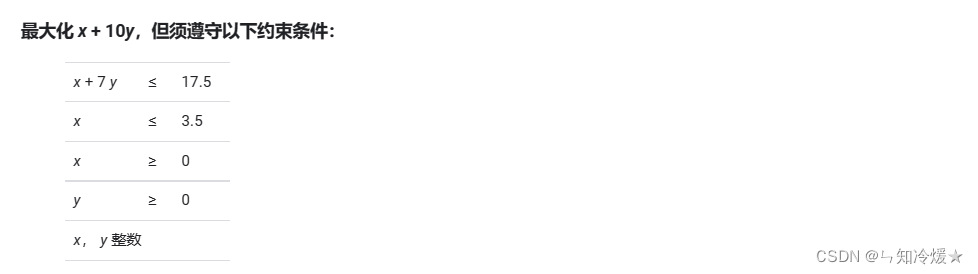
from ortools.linear_solver import pywraplpsolver = pywraplp.Solver.CreateSolver('SCIP')infinity = solver.infinity()# x and y are integer non-negative variables.# x和y都是整数变量,所以这里创建用到的是IntVar。x = solver.IntVar(0.0, infinity, 'x')y = solver.IntVar(0.0, infinity, 'y')print('Number of variables =', solver.NumVariables())# x + 7 * y <= 17.5.solver.Add(x + 7 * y <= 17.5)# x <= 3.5.solver.Add(x <= 3.5)print('Number of constraints =', solver.NumConstraints())# Maximize x + 10 * y.solver.Maximize(x + 10 * y)status = solver.Solve()if status == pywraplp.Solver.OPTIMAL: print('Solution:') print('Objective value =', solver.Objective().Value()) print('x =', x.solution_value()) print('y =', y.solution_value())else: print('The problem does not have an optimal solution.')输出结果: 即目标的最优值是23,发生在点x=3,y=2处。
from ortools.linear_solver import pywraplpsolver = pywraplp.Solver.CreateSolver('GLOP')输出结果:
在此示例中,有五个工作器(编号为 0-4)和四个任务(编号为 0-3)。下表显示了将工作器分配给任务的费用。
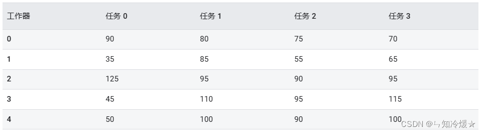
问题: 最多将每个工作器分配给一个任务,其中不包括两个工作器来执行相同的任务,同时最大限度地降低总费用。
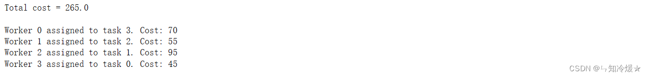
from ortools.sat.python import cp_modelmodel = cp_model.CpModel()costs = [ [90, 80, 75, 70], [35, 85, 55, 65], [125, 95, 90, 95], [45, 110, 95, 115], [50, 100, 90, 100],]num_workers = len(costs)num_tasks = len(costs[0])x = []for i in range(num_workers): t = [] for j in range(num_tasks): t.append(model.NewBoolVar(f'x[{i},{j}]')) x.append(t)# Each worker is assigned to at most one task.for i in range(num_workers): model.AddAtMostOne(x[i][j] for j in range(num_tasks))# Each task is assigned to exactly one worker.for j in range(num_tasks): model.AddExactlyOne(x[i][j] for i in range(num_workers))objective_terms = []for i in range(num_workers): for j in range(num_tasks): objective_terms.append(costs[i][j] * x[i][j])# 目标函数的值是求解器为值1分配的所有变量的总费用。model.Minimize(sum(objective_terms))solver = cp_model.CpSolver()status = solver.Solve(model)if status == cp_model.OPTIMAL or status == cp_model.FEASIBLE: print(f'Total cost = {solver.ObjectiveValue()}') print() for i in range(num_workers): for j in range(num_tasks): if solver.BooleanValue(x[i][j]): print( f'Worker {i} assigned to task {j} Cost = {costs[i][j]}')else: print('No solution found.')输出结果:
from ortools.linear_solver import pywraplpdef main(): # Data costs = [ [90, 80, 75, 70], [35, 85, 55, 65], [125, 95, 90, 95], [45, 110, 95, 115], [50, 100, 90, 100], ] # 工作器数量为5。 num_workers = len(costs) # 任务数量为4。 num_tasks = len(costs[0]) # Solver # Create the mip solver with the SCIP backend. # 创建求解器SCIP solver = pywraplp.Solver.CreateSolver('SCIP')# 如果没有获取到求解器,则返回为空。 if not solver: return # Variables # x[i, j] is an array of 0-1 variables, which will be 1 # if worker i is assigned to task j. x = [] # for i in range(num_workers): for j in range(num_tasks): # i: 工作器 j:任务 x[i, j] = solver.IntVar(0, 1, '') # Constraints # Each worker is assigned to at most 1 task. # 每一个工作器最多分配给一个任务 for i in range(num_workers): solver.Add(solver.Sum([x[i, j] for j in range(num_tasks)]) <= 1) # Each task is assigned to exactly one worker. # 每一个任务只能分配给一个工作器 for j in range(num_tasks): solver.Add(solver.Sum([x[i, j] for i in range(num_workers)]) == 1) # Objective objective_terms = [] for i in range(num_workers): for j in range(num_tasks): # 将花销和对应的变量相乘。 objective_terms.append(costs[i][j] * x[i, j]) # 最小化目标值 solver.Minimize(solver.Sum(objective_terms)) # Solve status = solver.Solve() # Print solution. if status == pywraplp.Solver.OPTIMAL or status == pywraplp.Solver.FEASIBLE: print(f'Total cost = {solver.Objective().Value()}\n') for i in range(num_workers): for j in range(num_tasks): # Test if x[i,j] is 1 (with tolerance for floating point arithmetic). if x[i, j].solution_value() > 0.5: print(f'Worker {i} assigned to task {j}.' + f' Cost: {costs[i][j]}') else: print('No solution found.')if __name__ == '__main__': main()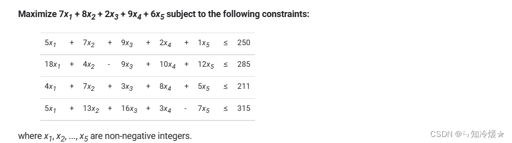
Notice: 与前边的MIP(混合整数规划)问题类似。
from ortools.linear_solver import pywraplp# 创建字典来将所有数据包含在内。def create_data_model(): """Stores the data for the problem.""" data = {} # 所有约束条件的系数列表 data['constraint_coeffs'] = [ [5, 7, 9, 2, 1], [18, 4, -9, 10, 12], [4, 7, 3, 8, 5], [5, 13, 16, 3, -7], ] # 所有约束条件的界限 data['bounds'] = [250, 285, 211, 315] # 目标条件的系数列表 data['obj_coeffs'] = [7, 8, 2, 9, 6] # 变量个数 data['num_vars'] = 5 # 约束条件数量 data['num_constraints'] = 4 return datadata = create_data_model()data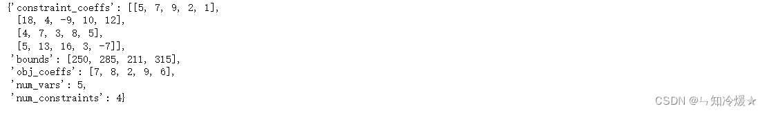
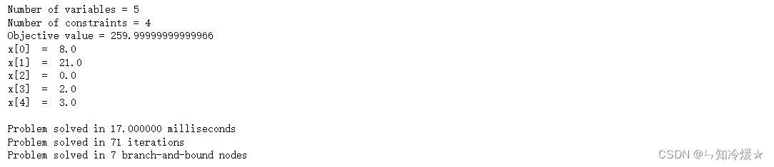
solver = pywraplp.Solver.CreateSolver('SCIP')# 在循环中定义示例的变量,对于变量较多的问题,这种方法比较容易infinity = solver.infinity()x = {}for j in range(data['num_vars']): x[j] = solver.IntVar(0, infinity, 'x[%i]' % j)print('Number of variables =', solver.NumVariables())# 约束条件数for i in range(data['num_constraints']):# 定义每一个约束的范围 constraint = solver.RowConstraint(0, data['bounds'][i], '') # 变量个数 for j in range(data['num_vars']): # 设置约束的系数,每次循环,给同一个变量添加所有的系数。 constraint.SetCoefficient(x[j], data['constraint_coeffs'][i][j])print('Number of constraints =', solver.NumConstraints())# In Python, you can also set the constraints as follows.# for i in range(data['num_constraints']):# constraint_expr = \# [data['constraint_coeffs'][i][j] * x[j] for j in range(data['num_vars'])]# solver.Add(sum(constraint_expr) <= data['bounds'][i])objective = solver.Objective()for j in range(data['num_vars']):# 将对应变量和对应的目标系数相乘,最后相加 objective.SetCoefficient(x[j], data['obj_coeffs'][j])# 目标函数最大化objective.SetMaximization()# In Python, you can also set the objective as follows.# obj_expr = [data['obj_coeffs'][j] * x[j] for j in range(data['num_vars'])]# solver.Maximize(solver.Sum(obj_expr))status = solver.Solve()if status == pywraplp.Solver.OPTIMAL: print('Objective value =', solver.Objective().Value()) for j in range(data['num_vars']): print(x[j].name(), ' = ', x[j].solution_value()) print() print('Problem solved in %f milliseconds' % solver.wall_time()) print('Problem solved in %d iterations' % solver.iterations()) print('Problem solved in %d branch-and-bound nodes' % solver.nodes())else: print('The problem does not have an optimal solution.')输出结果:
参考文章:
OR-Tools官网.
OR-Tools 示例.
MPSolver 接口-----用于解决线性规划和混合整数规划问题.
高级LP求解.
哪有什么永恒,珍惜当下!
来源地址:https://blog.csdn.net/weixin_42475060/article/details/128315221
--结束END--
本文标题: OR-Tools工具介绍以及实战(从入门到超神Python版)
本文链接: https://www.lsjlt.com/news/391615.html(转载时请注明来源链接)
有问题或投稿请发送至: 邮箱/279061341@qq.com QQ/279061341
下载Word文档到电脑,方便收藏和打印~
2024-03-01
2024-03-01
2024-03-01
2024-02-29
2024-02-29
2024-02-29
2024-02-29
2024-02-29
2024-02-29
2024-02-29
回答
回答
回答
回答
回答
回答
回答
回答
回答
回答


官方手机版

微信公众号

商务合作


0