本文参加新星计划人工智能(PyTorch)赛道：https://bbs.csdn.net/topics/613989052

目录

一、项目介绍

二、准备工作

三、实验过程

3.1数据预处理

3.2拆分数据集

3.3构建PyTorch模型

3.3.1.数据转换

3.3.2定义模型架构

3.3.3定义损失准则和优化器

3.3.4创建数据加载器

3.3.5训练模型

四、原理讲解

五、补充

一、项目介绍

        在此项目中，目的是预测爱荷华州Ames的房价，给定81个特征，描述了房子、面积、土地、基础设施、公共设施等。埃姆斯数据集具有分类和连续特征的良好组合，大小适中，也许最重要的是，它不像其他类似的数据集（如波士顿住房）那样存在潜在的红线或数据输入问题。在这里我将主要讨论PyTorch建模的相关方面，作为一点额外的内容，我还将演示PyTorch中开发的模型的神经元重要性。你可以在PyTorch中尝试不同的网络架构或模型类型。本项目中的重点是方法论，而不是详尽地寻找最佳解决方案。

二、准备工作

为了准备这个项目，我们首先需要下载数据，并通过以下步骤进行一些预处理。

from sklearn.datasets import fetch_openmldata = fetch_openml(data_id=42165, as_frame=True)

关于该数据集的完整描述，你可以去该网址查看：https://www.openml.org/d/42165。

查看数据特征

import pandas as pddata_ames = pd.DataFrame(data.data, columns=data.feature_names)data_ames['SalePrice'] = data.targetdata_ames.info()

下面是DataFrame的信息

RangeIndex: 1460 entries, 0 to 1459Data columns (total 81 columns):Id               1460 non-null float64MSSubClass       1460 non-null float64MSZoning         1460 non-null objectLotFrontage      1201 non-null float64LotArea          1460 non-null float64Street           1460 non-null objectAlley            91 non-null objectLotShape         1460 non-null objectLandContour      1460 non-null objectUtilities        1460 non-null objectLotConfig        1460 non-null objectLandSlope        1460 non-null objectNeighborhood     1460 non-null objectCondition1       1460 non-null objectCondition2       1460 non-null objectBldgType         1460 non-null objectHouseStyle       1460 non-null objectOverallQual      1460 non-null float64OverallCond      1460 non-null float64YearBuilt        1460 non-null float64YearRemodAdd     1460 non-null float64RoofStyle        1460 non-null objectRoofMatl         1460 non-null objectExterior1st      1460 non-null objectExterior2nd      1460 non-null objectMasVnrType       1452 non-null objectMasVnrArea       1452 non-null float64ExterQual        1460 non-null objectExterCond        1460 non-null objectFoundation       1460 non-null objectBsmtQual         1423 non-null objectBsmtCond         1423 non-null objectBsmtExposure     1422 non-null objectBsmtFinType1     1423 non-null objectBsmtFinSF1       1460 non-null float64BsmtFinType2     1422 non-null objectBsmtFinSF2       1460 non-null float64BsmtUnfSF        1460 non-null float64TotalBsmtSF      1460 non-null float64Heating          1460 non-null objectHeatingQC        1460 non-null objectCentralair       1460 non-null objectElectrical       1459 non-null object1stFlrSF         1460 non-null float642ndFlrSF         1460 non-null float64LowQualFinSF     1460 non-null float64GrLivArea        1460 non-null float64BsmtFullBath     1460 non-null float64BsmtHalfBath     1460 non-null float64FullBath         1460 non-null float64HalfBath         1460 non-null float64BedroomAbvGr     1460 non-null float64KitchenAbvGr     1460 non-null float64KitchenQual      1460 non-null objectTotRmsAbvGrd     1460 non-null float64Functional       1460 non-null objectFireplaces       1460 non-null float64FireplaceQu      770 non-null objectGarageType       1379 non-null objectGarageYrBlt      1379 non-null float64GarageFinish     1379 non-null objectGarageCars       1460 non-null float64GarageArea       1460 non-null float64GarageQual       1379 non-null objectGarageCond       1379 non-null objectPavedDrive       1460 non-null objectWoodDeckSF       1460 non-null float64OpenPorchSF      1460 non-null float64EnclosedPorch    1460 non-null float643SsnPorch        1460 non-null float64ScreenPorch      1460 non-null float64PoolArea         1460 non-null float64PoolQC           7 non-null objectFence            281 non-null objectMiscFeature      54 non-null objectMiscVal          1460 non-null float64MoSold           1460 non-null float64YrSold           1460 non-null float64SaleType         1460 non-null objectSaleCondition    1460 non-null objectSalePrice        1460 non-null float64dtypes: float64(38), object(43)memory usage: 924.0+ KB

接下来，我们还将使用一个库，即 captum，它可以检查 PyTorch 模型的特征和神经元重要性。

pip install captum

 在做完这些准备工作后，我们来看看如何预测房价。

三、实验过程

3.1数据预处理

        在这里，首先要进行数据缩放处理，因为所有的变量都有不同的尺度。分类变量需要转换为数值类型，以便将它们输入到我们的模型中。我们可以选择一热编码，即我们为每个分类因子创建哑变量，或者是序数编码，即我们对所有因子进行编号，并用这些数字替换字符串。我们可以像其他浮动变量一样将虚拟变量送入，而序数编码则需要使用嵌入，即线性神经网络投影，在多维空间中对类别进行重新排序。我们在这里采取嵌入的方式。

import numpy as npfrom cateGory_encoders.ordinal import OrdinalEncoderfrom sklearn.preprocessing import StandardScalernum_cols = list(data_ames.select_dtypes(include='float'))cat_cols = list(data_ames.select_dtypes(include='object'))ordinal_encoder = OrdinalEncoder().fit(    data_ames[cat_cols])standard_scaler = StandardScaler().fit(    data_ames[num_cols])X = pd.DataFrame(    data=np.column_stack([        ordinal_encoder.transfORM(data_ames[cat_cols]),        standard_scaler.transform(data_ames[num_cols])    ]),    columns=cat_cols + num_cols)

3.2拆分数据集

       在构建模型之前，我们需要将数据拆分为训练集和测试集。在这里，我们添加了一个数值变量的分层。这可以确保不同的部分（其中五个）在训练集和测试集中都以同等的数量包含。

np.random.seed(12)  from sklearn.model_selection import train_test_splitbins = 5sale_price_bins = pd.qcut(    X['SalePrice'], q=bins, labels=list(range(bins)))X_train, X_test, y_train, y_test = train_test_split(    X.drop(columns='SalePrice'),    X['SalePrice'],    random_state=12,    stratify=sale_price_bins)

3.3构建PyTorch模型

        接下来开始建立我们的PyTorch模型。我们将使用PyTorch实现一个具有批量输入的神经网络回归，具体将涉及以下步骤。

• 1. 将数据转换为Torch tensors
• 2. 定义模型结构
• 3. 定义损失标准和优化器。
• 4. 创建一个批次的数据加载器
• 5. 跑步训练

3.3.1.数据转换

首先将数据转换为torch tensors

from torch.autograd import Variable num_features = list(    set(num_cols) - set(['SalePrice', 'Id']))X_train_num_pt = Variable(    torch.cuda.FloatTensor(        X_train[num_features].values    ))X_train_cat_pt = Variable(    torch.cuda.LongTensor(        X_train[cat_cols].values    ))y_train_pt = Variable(    torch.cuda.FloatTensor(y_train.values)).view(-1, 1)X_test_num_pt = Variable(    torch.cuda.FloatTensor(        X_test[num_features].values    ))X_test_cat_pt = Variable(   torch.cuda.LongTensor(        X_test[cat_cols].values    ).long())y_test_pt = Variable(    torch.cuda.FloatTensor(y_test.values)).view(-1, 1)

        这可以确保我们将数字和分类数据加载到单独的变量中，类似于NumPy。如果你把数据类型混合在一个变量（数组/矩阵）中，它们就会变成对象。我们希望把数值变量弄成浮点数，把分类变量弄成长（或int），索引我们的类别。我们还将训练集和测试集分开。显然，一个ID变量在模型中不应该是重要的。在最坏的情况下，如果ID与目标有任何相关性，它可能会引入目标泄漏。我们已经把它从这一步的处理中删除了。

3.3.2定义模型架构

class RegressionModel(torch.nn.Module):       def __init__(self, X, num_cols, cat_cols, device=torch.device('cuda'), embed_dim=2, hidden_layer_dim=2, p=0.5):         super(RegressionModel, self).__init__()         self.num_cols = num_cols        self.cat_cols = cat_cols        self.embed_dim = embed_dim        self.hidden_layer_dim = hidden_layer_dim                self.embeddings = [            torch.nn.Embedding(                num_embeddings=len(X[col].unique()),                embedding_dim=embed_dim            ).to(device)            for col in cat_cols        ]        hidden_dim = len(num_cols) + len(cat_cols) * embed_dim,                # hidden layer        self.hidden = torch.nn.Linear(torch.IntTensor(hidden_dim), hidden_layer_dim).to(device)        self.dropout_layer = torch.nn.Dropout(p=p).to(device)        self.hidden_act = torch.nn.ReLU().to(device)                # output layer        self.output = torch.nn.Linear(hidden_layer_dim, 1).to(device)        def forward(self, num_inputs, cat_inputs):        '''Forward method with two input variables -        numeric and categorical.        '''        cat_x = [            torch.squeeze(embed(cat_inputs[:, i] - 1))            for i, embed in enumerate(self.embeddings)        ]        x = torch.cat(cat_x + [num_inputs], dim=1)        x = self.hidden(x)        x = self.dropout_layer(x)        x = self.hidden_act(x)        y_pred = self.output(x)        return y_predhouse_model = RegressionModel(    data_ames, num_features, cat_cols)

        我们在两个线性层（上的激活函数是整流线性单元激活（ReLU）函数。这里需要注意的是，我们不可能将相同的架构（很容易）封装成一个顺序模型，因为分类和数值类型上发生的操作不同。

3.3.3定义损失准则和优化器

        接下来，定义损失准则和优化器。我们将均方误差（MSE）作为损失，随机梯度下降作为我们的优化算法。

criterion = torch.nn.MSELoss().to(device)optimizer = torch.optim.SGD(house_model.parameters(), lr=0.001)

3.3.4创建数据加载器

现在，创建一个数据加载器，每次输入一批数据。

data_batch = torch.utils.data.TensorDataset(    X_train_num_pt, X_train_cat_pt, y_train_pt)dataloader = torch.utils.data.DataLoader(    data_batch, batch_size=10, shuffle=True)

我们设置了10个批次的大小，接下来我们可以进行训练了。

3.3.5.训练模型

       基本上，我们要在epoch上循环，在每个epoch内推理出性能，计算出误差，优化器根据误差进行调整。这是在没有训练的内循环的情况下，在epochs上的循环。

from tqdm.notebook import trangetrain_losses, test_losses = [], []n_epochs = 30for epoch in trange(n_epochs):    train_loss, test_loss = 0, 0      # print the errors in training and test:    if epoch % 10 == 0 :        print(            'Epoch: {}/{}\t'.format(epoch, 1000),            'Training Loss: {:.3f}\t'.format(                train_loss / len(dataloader)            ),            'Test Loss: {:.3f}'.format(                test_loss / len(dataloader)            )        )

 训练是在这个循环里面对所有批次的训练数据进行的。

for (x_train_num_batch,x_train_cat_batch,y_train_batch) in dataloader:        (x_train_num_batch,x_train_cat_batch, y_train_batch) = (                x_train_num_batch.to(device),                x_train_cat_batch.to(device),                y_train_batch.to(device))        pred_ytrain = house_model.forward(x_train_num_batch, x_train_cat_batch)        loss = torch.sqrt(criterion(pred_ytrain, y_train_batch))         optimizer.zero_grad()         loss.backward()         optimizer.step()        train_loss += loss.item()        with torch.no_grad():            house_model.eval()            pred_ytest = house_model.forward(X_test_num_pt, X_test_cat_pt)            test_loss += torch.sqrt(criterion(pred_ytest, y_test_pt))        train_losses.append(train_loss / len(dataloader))        test_losses.append(test_loss / len(dataloader))

训练结果如下：

我们取 nn.MSELoss 的平方根，因为 PyTorch 中 nn.MSELoss 的定义如下：

((input-target)**2).mean()

绘制一下我们的模型在训练期间对训练和验证数据集的表现。

plt.plot(    np.array(train_losses).reshape((n_epochs, -1)).mean(axis=1),    label='Training loss')plt.plot(    np.array(test_losses).reshape((n_epochs, -1)).mean(axis=1),    label='Validation loss')plt.legend(frameon=False)plt.xlabel('epochs')plt.ylabel('MSE')

        在我们的验证损失停止下降之前，我们及时停止了训练。我们还可以对目标变量进行排序和bin，并将预测结果与之对比绘制，以便了解模型在整个房价范围内的表现。这是为了避免回归中的情况，尤其是用MSE作为损失，即你只对一个中值范围的预测很好，接近平均值，但对其他任何东西都做得不好。

        我们可以看到，事实上，这个模型在整个房价范围内的预测非常接近。事实上，我们得到的Spearman秩相关度约为93%，具有非常高的显著性，这证实了这个模型的表现具有很高的准确性。

四、原理讲解

        深度学习神经网络框架使用不同的优化算法。其中流行的有随机梯度下降（SGD）、均方根推进（RMSProp）和自适应矩估计（ADAM）。我们定义了随机梯度下降作为我们的优化算法。另外，我们还可以定义其他优化器。

opt_SGD = torch.optim.SGD(net_SGD.parameters(), lr=LR)opt_Momentum = torch.optim.SGD(net_Momentum.parameters(), lr=LR, momentum=0.6)opt_RMSprop = torch.optim.RMSprop(net_RMSprop.parameters(), lr=LR, alpha=0.1)opt_Adam = torch.optim.Adam(net_Adam.parameters(), lr=LR, betas=(0.8, 0.98))

        SGD的工作原理与梯度下降相同，只是它每次只在一个例子上工作。有趣的是，收敛性与梯度下降相似，并且更容易占用计算机内存。

        RMSProp的工作原理是根据梯度符号来调整算法的学习率。最简单的变体是检查最后两个梯度符号，然后调整学习率，如果它们相同，则增加一个分数，如果它们不同，则减少一个分数。

        ADAM是最流行的优化器之一。它是一种自适应学习算法，根据梯度的第一和第二时刻改变学习率。

        Captum是一个工具，可以帮助我们了解在数据集上学习的神经网络模型的来龙去脉。它可以帮助我们学习以下内容。

• 特征重要性

• 层级重要性

• 神经元的重要性

        这在学习可解释的神经网络中是非常重要的。在这里，综合梯度已经被应用于理解特征重要性。之后，还用层传导法来证明神经元的重要性。

五、补充

        既然我们已经定义并训练了我们的神经网络，那么让我们使用 captum 库找到重要的特征和神经元。

from captum.attr import (    IntegratedGradients,    LayerConductance,    NeuronConductance)house_model.cpu()for embedding in house_model.embeddings:    embedding.cpu()house_model.cpu()ing_house = IntegratedGradients(forward_func=house_model.forward, )#X_test_cat_pt.requires_grad_()X_test_num_pt.requires_grad_()attr, delta = ing_house.attribute( X_test_num_pt.cpu(), target=None, return_convergence_delta=True, additional_forward_args=X_test_cat_pt.cpu())attr = attr.detach().numpy()

 现在，我们有了一个NumPy的特征重要性数组。层和神经元的重要性也可以用这个工具获得。让我们来看看我们第一层的神经元importances。我们可以传递house_model.act1，这是第一层线性层上面的ReLU激活函数。

cond_layer1 = LayerConductance(house_model, house_model.act1)cond_vals = cond_layer1.attribute(X_test, target=None)cond_vals = cond_vals.detach().numpy()df_neuron = pd.DataFrame(data = np.mean(cond_vals, axis=0), columns=['Neuron Importance'])df_neuron['Neuron'] = range(10)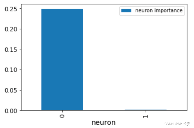

这张图显示了神经元的重要性。显然，一个神经元就是不重要的。我们还可以通过对之前得到的NumPy数组进行排序，看到最重要的变量。

df_feat = pd.DataFrame(np.mean(attr, axis=0), columns=['feature importance'] )df_feat['features'] = num_featuresdf_feat.sort_values(    by='feature importance', ascending=False).head(10)

 这里列出了10个最重要的变量

        通常情况下，特征导入可以帮助我们既理解模型，又修剪我们的模型，使其变得不那么复杂（希望减少过度拟合）。

来源地址：https://blog.csdn.net/zxb_1222/article/details/129756586