文章目录

• LSTM 时间序列预测
• • 股票预测案例
  • • 数据特征
    • 对收盘价(Close)单特征进行预测
    • • 1. 导入数据
      • 2. 将股票数据收盘价(Close)进行可视化展示
      • 3. 特征工程
      • 4. 数据集制作
      • 5. 模型构建
      • 6. 模型训练
      • 7. 模型结果可视化
      • 8. 模型验证
    • 完整代码

LSTM 时间序列预测

股票预测案例

数据特征

• Date：日期
• Open：开盘价
• High：最高价
• Low：最低价
• Close：收盘价
• Adj Close：调整后的收盘价
• Volume：交易量

对收盘价(Close)单特征进行预测

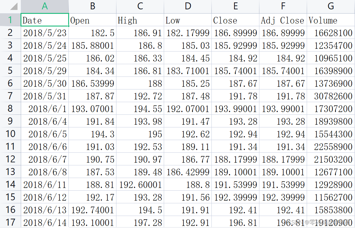
利用前n天的数据预测第n+1天的数据。

1. 导入数据

import numpy as npimport pandas as pdimport matplotlib.pyplot as pltimport seaborn as snsfrom sklearn.preprocessing import MinMaxScalerfilepath = 'D:/pythonProjects/LSTM/data/rlData.csv'data = pd.read_csv(filepath)# 将数据按照日期进行排序，确保时间序列递增data = data.sort_values('Date')# 打印前几条数据print(data.head())# 打印维度print(data.shape)

2. 将股票数据收盘价(Close)进行可视化展示

# 设置画布大小plt.figure(figsize=(15, 9))plt.plot(data[['Close']])plt.xticks(range(0, data.shape[0], 20), data['Date'].loc[::20], rotation=45)plt.title("****** Stock Price", fontsize=18, fontweight='bold')plt.xlabel('Date', fontsize=18)plt.ylabel('Close Price (USD)', fontsize=18)plt.savefig('StockPrice.jpg')plt.show()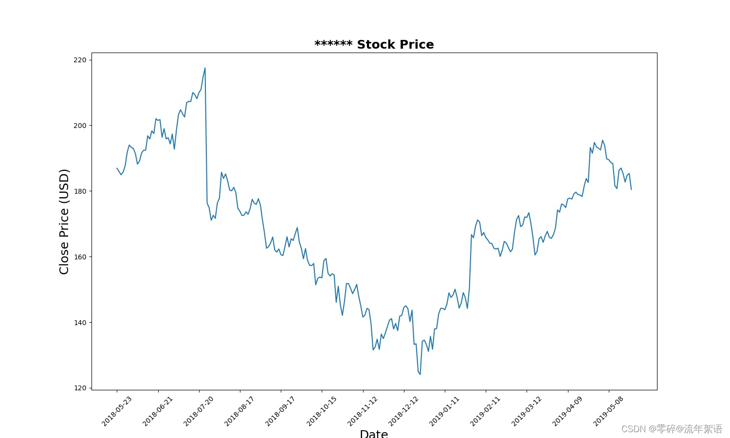

3. 特征工程

# 选取Close作为特征price = data[['Close']]# 打印相关信息print(price.info())

打印结果如下：Int64Index: 252 entries, 0 to 251Data columns (total 1 columns): #   Column  Non-Null Count  Dtype  ---  ------  --------------  -----   0   Close   252 non-null    float64dtypes: float64(1)memory usage: 3.9 KBNone可以看出：price为DataFrame对象，以及其的结构和占用内存等信息

# 进行不同的数据缩放，将数据缩放到-1和1之间，归一化操作scaler = MinMaxScaler(feature_range=(-1, 1))price['Close'] = scaler.fit_transfORM(price['Close'].values.reshape(-1, 1))print(price['Close'].shape)

打印结果如下：0      0.3450341      0.3242722      0.3026543      0.3202064      0.361515         ...   247    0.310788248    0.255565249    0.300514250    0.311216251    0.207192Name: Close, Length: 252, dtype: float64Int64Index: 252 entries, 0 to 251Series name: CloseNon-Null Count  Dtype  --------------  -----  252 non-null    float64dtypes: float64(1)memory usage: 3.9 KBNone(252,)可以看出：price['Close']的值，price['Close']为Series结构，price['Close']的结构为(252,)

4. 数据集制作

# 今天的收盘价预测明天的收盘价# lookback表示观察的跨度def split_data(stock, lookback):# 将stock转化为ndarray类型    data_raw = stock.to_numpy()    data = []    # you can free play（seq_length）    # 将data按lookback分组，data为长度为lookback的list    for index in range(len(data_raw) - lookback):        data.append(data_raw[index: index + lookback])    data = np.array(data);    print(type(data))  # (232, 20, 1)    # 按照8:2进行训练集、测试集划分    test_set_size = int(np.round(0.2 * data.shape[0]))    train_set_size = data.shape[0] - (test_set_size)    x_train = data[:train_set_size, :-1, :]    y_train = data[:train_set_size, -1, :]    x_test = data[train_set_size:, :-1]    y_test = data[train_set_size:, -1, :]    return [x_train, y_train, x_test, y_test]lookback = 20x_train, y_train, x_test, y_test = split_data(price, lookback)print('x_train.shape = ', x_train.shape)print('y_train.shape = ', y_train.shape)print('x_test.shape = ', x_test.shape)print('y_test.shape = ', y_test.shape)

打印结果如下：x_train.shape =  (186, 19, 1)y_train.shape =  (186, 1)x_test.shape =  (46, 19, 1)y_test.shape =  (46, 1)

5. 模型构建

import torchimport torch.nn as nnx_train = torch.from_numpy(x_train).type(torch.Tensor)x_test = torch.from_numpy(x_test).type(torch.Tensor)# 真实的数据y_train_lstm = torch.from_numpy(y_train).type(torch.Tensor)y_test_lstm = torch.from_numpy(y_test).type(torch.Tensor)y_train_gru = torch.from_numpy(y_train).type(torch.Tensor)y_test_gru = torch.from_numpy(y_test).type(torch.Tensor)# 输入的维度为1，只有Close收盘价input_dim = 1# 隐藏层特征的维度hidden_dim = 32# 循环的layersnum_layers = 2# 预测后一天的收盘价output_dim = 1num_epochs = 100class LSTM(nn.Module):    def __init__(self, input_dim, hidden_dim, num_layers, output_dim):        super(LSTM, self).__init__()        self.hidden_dim = hidden_dim        self.num_layers = num_layers        self.lstm = nn.LSTM(input_dim, hidden_dim, num_layers, batch_first=True)        self.fc = nn.Linear(hidden_dim, output_dim)    def forward(self, x):        h0 = torch.zeros(self.num_layers, x.size(0), self.hidden_dim).requires_grad_()        c0 = torch.zeros(self.num_layers, x.size(0), self.hidden_dim).requires_grad_()        out, (hn, cn) = self.lstm(x, (h0.detach(), c0.detach()))        out = self.fc(out[:, -1, :])        return outmodel = LSTM(input_dim=input_dim, hidden_dim=hidden_dim, output_dim=output_dim, num_layers=num_layers)criterion = torch.nn.MSELoss()optimiser = torch.optim.Adam(model.parameters(), lr=0.01)

6. 模型训练

import timehist = np.zeros(num_epochs)start_time = time.time()lstm = []for t in range(num_epochs):    y_train_pred = model(x_train)    loss = criterion(y_train_pred, y_train_lstm)    print("Epoch ", t, "MSE: ", loss.item())    hist[t] = loss.item()    optimiser.zero_grad()    loss.backward()    optimiser.step()training_time = time.time() - start_timeprint("Training time: {}".format(training_time))predict = pd.DataFrame(scaler.inverse_transform(y_train_pred.detach().numpy()))print(predict)  # 预测值original = pd.DataFrame(scaler.inverse_transform(y_train_lstm.detach().numpy()))print(original)  # 真实值

打印结果如下：其中预测值每次运行可能会有一定的差距，但不影响最后的结果。torch.Size([186, 1])Epoch  0 MSE:  0.19840142130851746torch.Size([186, 1])Epoch  1 MSE:  0.17595666646957397torch.Size([186, 1])Epoch  2 MSE:  0.1369851976633072torch.Size([186, 1])..          ...Epoch  96 MSE:  0.008701297454535961torch.Size([186, 1])Epoch  97 MSE:  0.008698086254298687torch.Size([186, 1])Epoch  98 MSE:  0.008688708767294884torch.Size([186, 1])Epoch  99 MSE:  0.008677813224494457Training time: 3.884610414505005              00    196.6549991    201.0952912    200.1985633    200.4940034    195.120148..          ...181  171.398987182  171.508194183  172.992401184  169.850494185  165.566605[186 rows x 1 columns]              00    201.9999851    201.5000152    201.7400053    196.3500064    198.999985..          ...181  171.919998182  173.369995183  170.169998184  165.979996185  160.470001[186 rows x 1 columns]

7. 模型结果可视化

import seaborn as snssns.set_style("darkgrid")fig = plt.figure()fig.subplots_adjust(hspace=0.2, wspace=0.2)plt.subplot(1, 2, 1)ax = sns.lineplot(x = original.index, y = original[0], label="Data", color='royalblue')ax = sns.lineplot(x = predict.index, y = predict[0], label="Training Prediction (LSTM)", color='tomato')print(predict.index)print("aaaa")print(predict[0])ax.set_title('Stock price', size = 14, fontweight='bold')ax.set_xlabel("Days", size = 14)ax.set_ylabel("Cost (USD)", size = 14)ax.set_xticklabels('', size=10)plt.subplot(1, 2, 2)ax = sns.lineplot(data=hist, color='royalblue')ax.set_xlabel("Epoch", size = 14)ax.set_ylabel("Loss", size = 14)ax.set_title("Training Loss", size = 14, fontweight='bold')fig.set_figheight(6)fig.set_figwidth(16)plt.show()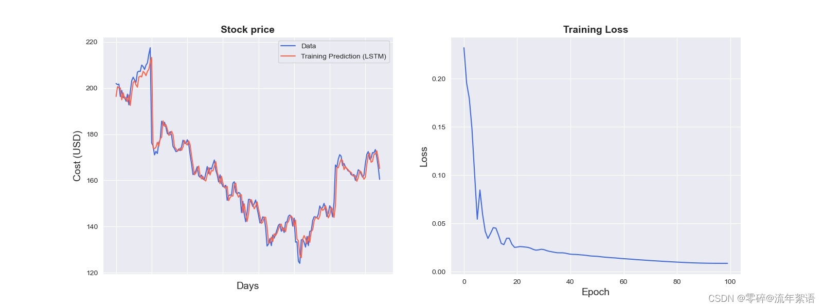

8. 模型验证

实际上是对结果的总结及进一步说明。

import math, timefrom sklearn.metrics import mean_squared_error# make predictionsy_test_pred = model(x_test)# invert predictionsy_train_pred = scaler.inverse_transform(y_train_pred.detach().numpy())y_train = scaler.inverse_transform(y_train_lstm.detach().numpy())y_test_pred = scaler.inverse_transform(y_test_pred.detach().numpy())y_test = scaler.inverse_transform(y_test_lstm.detach().numpy())# calculate root mean squared errortrainScore = math.sqrt(mean_squared_error(y_train[:,0], y_train_pred[:,0]))print('Train Score: %.2f RMSE' % (trainScore))testScore = math.sqrt(mean_squared_error(y_test[:,0], y_test_pred[:,0]))print('Test Score: %.2f RMSE' % (testScore))lstm.append(trainScore)lstm.append(testScore)lstm.append(training_time)# shift train predictions for plottingtrainPredictPlot = np.empty_like(price)trainPredictPlot[:, :] = np.nantrainPredictPlot[lookback:len(y_train_pred)+lookback, :] = y_train_pred# shift test predictions for plottingtestPredictPlot = np.empty_like(price)testPredictPlot[:, :] = np.nantestPredictPlot[len(y_train_pred)+lookback-1:len(price)-1, :] = y_test_predoriginal = scaler.inverse_transform(price['Close'].values.reshape(-1,1))predictions = np.append(trainPredictPlot, testPredictPlot, axis=1)predictions = np.append(predictions, original, axis=1)result = pd.DataFrame(predictions)import plotly.express as pximport plotly.graph_objects as Gofig = go.Figure()fig.add_trace(go.Scatter(go.Scatter(x=result.index, y=result[0],                    mode='lines',                    name='Train prediction')))fig.add_trace(go.Scatter(x=result.index, y=result[1],                    mode='lines',                    name='Test prediction'))fig.add_trace(go.Scatter(go.Scatter(x=result.index, y=result[2],                    mode='lines',                    name='Actual Value')))fig.update_layout(    xaxis=dict(        showline=True,        showgrid=True,        showticklabels=False,        linecolor='white',        linewidth=2    ),    yaxis=dict(        title_text='Close (USD)',        titlefont=dict(            family='Rockwell',            size=12,            color='white',        ),        showline=True,        showgrid=True,        showticklabels=True,        linecolor='white',        linewidth=2,        ticks='outside',        tickfont=dict(            family='Rockwell',            size=12,            color='white',        ),    ),    showlegend=True,    template = 'plotly_dark')annotations = []annotations.append(dict(xref='paper', yref='paper', x=0.0, y=1.05,  xanchor='left', yanchor='bottom',  text='Results (LSTM)',  font=dict(family='Rockwell',            size=26,            color='white'),  showarrow=False))fig.update_layout(annotations=annotations)fig.show()

完整代码

import numpy as npimport pandas as pdimport matplotlib.pyplot as pltimport seaborn as snsfilepath = 'D:/PythonProjects/LSTM/data/rlData.csv'data = pd.read_csv(filepath)data = data.sort_values('Date')print(data.head())print(data.shape)sns.set_style("darkgrid")plt.figure(figsize=(15, 9))plt.plot(data[['Close']])plt.xticks(range(0, data.shape[0], 20), data['Date'].loc[::20], rotation=45)plt.title("****** Stock Price", fontsize=18, fontweight='bold')plt.xlabel('Date', fontsize=18)plt.ylabel('Close Price (USD)', fontsize=18)plt.show()# 1.特征工程# 选取Close作为特征price = data[['Close']]print(price.info())from sklearn.preprocessing import MinMaxScaler# 进行不同的数据缩放，将数据缩放到-1和1之间scaler = MinMaxScaler(feature_range=(-1, 1))price['Close'] = scaler.fit_transform(price['Close'].values.reshape(-1, 1))print(price['Close'].shape)# 2.数据集制作# 今天的收盘价预测明天的收盘价# lookback表示观察的跨度def split_data(stock, lookback):    data_raw = stock.to_numpy()    data = []    # print(data)    # you can free play（seq_length）    for index in range(len(data_raw) - lookback):        data.append(data_raw[index: index + lookback])    data = np.array(data);    test_set_size = int(np.round(0.2 * data.shape[0]))    train_set_size = data.shape[0] - (test_set_size)    x_train = data[:train_set_size, :-1, :]    y_train = data[:train_set_size, -1, :]    x_test = data[train_set_size:, :-1]    y_test = data[train_set_size:, -1, :]    return [x_train, y_train, x_test, y_test]lookback = 20x_train, y_train, x_test, y_test = split_data(price, lookback)print('x_train.shape = ', x_train.shape)print('y_train.shape = ', y_train.shape)print('x_test.shape = ', x_test.shape)print('y_test.shape = ', y_test.shape)# 注意：PyTorch的nn.LSTM input shape=(seq_length, batch_size, input_size)# 3.模型构建 —— LSTMimport torchimport torch.nn as nnx_train = torch.from_numpy(x_train).type(torch.Tensor)x_test = torch.from_numpy(x_test).type(torch.Tensor)y_train_lstm = torch.from_numpy(y_train).type(torch.Tensor)y_test_lstm = torch.from_numpy(y_test).type(torch.Tensor)y_train_gru = torch.from_numpy(y_train).type(torch.Tensor)y_test_gru = torch.from_numpy(y_test).type(torch.Tensor)# 输入的维度为1，只有Close收盘价input_dim = 1# 隐藏层特征的维度hidden_dim = 32# 循环的layersnum_layers = 2# 预测后一天的收盘价output_dim = 1num_epochs = 100class LSTM(nn.Module):    def __init__(self, input_dim, hidden_dim, num_layers, output_dim):        super(LSTM, self).__init__()        self.hidden_dim = hidden_dim        self.num_layers = num_layers        self.lstm = nn.LSTM(input_dim, hidden_dim, num_layers, batch_first=True)        self.fc = nn.Linear(hidden_dim, output_dim)    def forward(self, x):        h0 = torch.zeros(self.num_layers, x.size(0), self.hidden_dim).requires_grad_()        c0 = torch.zeros(self.num_layers, x.size(0), self.hidden_dim).requires_grad_()        out, (hn, cn) = self.lstm(x, (h0.detach(), c0.detach()))        out = self.fc(out[:, -1, :])        return outmodel = LSTM(input_dim=input_dim, hidden_dim=hidden_dim, output_dim=output_dim, num_layers=num_layers)criterion = torch.nn.MSELoss()optimiser = torch.optim.Adam(model.parameters(), lr=0.01)# 4.模型训练import timehist = np.zeros(num_epochs)start_time = time.time()lstm = []for t in range(num_epochs):    y_train_pred = model(x_train)    loss = criterion(y_train_pred, y_train_lstm)    print("Epoch ", t, "MSE: ", loss.item())    hist[t] = loss.item()    optimiser.zero_grad()    loss.backward()    optimiser.step()training_time = time.time() - start_timeprint("Training time: {}".format(training_time))# 5.模型结果可视化predict = pd.DataFrame(scaler.inverse_transform(y_train_pred.detach().numpy()))original = pd.DataFrame(scaler.inverse_transform(y_train_lstm.detach().numpy()))import seaborn as snssns.set_style("darkgrid")fig = plt.figure()fig.subplots_adjust(hspace=0.2, wspace=0.2)plt.subplot(1, 2, 1)ax = sns.lineplot(x = original.index, y = original[0], label="Data", color='royalblue')ax = sns.lineplot(x = predict.index, y = predict[0], label="Training Prediction (LSTM)", color='tomato')# print(predict.index)# print(predict[0])ax.set_title('Stock price', size = 14, fontweight='bold')ax.set_xlabel("Days", size = 14)ax.set_ylabel("Cost (USD)", size = 14)ax.set_xticklabels('', size=10)plt.subplot(1, 2, 2)ax = sns.lineplot(data=hist, color='royalblue')ax.set_xlabel("Epoch", size = 14)ax.set_ylabel("Loss", size = 14)ax.set_title("Training Loss", size = 14, fontweight='bold')fig.set_figheight(6)fig.set_figwidth(16)plt.show()# 6.模型验证# print(x_test[-1])import math, timefrom sklearn.metrics import mean_squared_error# make predictionsy_test_pred = model(x_test)# invert predictionsy_train_pred = scaler.inverse_transform(y_train_pred.detach().numpy())y_train = scaler.inverse_transform(y_train_lstm.detach().numpy())y_test_pred = scaler.inverse_transform(y_test_pred.detach().numpy())y_test = scaler.inverse_transform(y_test_lstm.detach().numpy())# calculate root mean squared errortrainScore = math.sqrt(mean_squared_error(y_train[:,0], y_train_pred[:,0]))print('Train Score: %.2f RMSE' % (trainScore))testScore = math.sqrt(mean_squared_error(y_test[:,0], y_test_pred[:,0]))print('Test Score: %.2f RMSE' % (testScore))lstm.append(trainScore)lstm.append(testScore)lstm.append(training_time)# In[40]:# shift train predictions for plottingtrainPredictPlot = np.empty_like(price)trainPredictPlot[:, :] = np.nantrainPredictPlot[lookback:len(y_train_pred)+lookback, :] = y_train_pred# shift test predictions for plottingtestPredictPlot = np.empty_like(price)testPredictPlot[:, :] = np.nantestPredictPlot[len(y_train_pred)+lookback-1:len(price)-1, :] = y_test_predoriginal = scaler.inverse_transform(price['Close'].values.reshape(-1,1))predictions = np.append(trainPredictPlot, testPredictPlot, axis=1)predictions = np.append(predictions, original, axis=1)result = pd.DataFrame(predictions)import plotly.express as pximport plotly.graph_objects as gofig = go.Figure()fig.add_trace(go.Scatter(go.Scatter(x=result.index, y=result[0],                    mode='lines',                    name='Train prediction')))fig.add_trace(go.Scatter(x=result.index, y=result[1],                    mode='lines',                    name='Test prediction'))fig.add_trace(go.Scatter(go.Scatter(x=result.index, y=result[2],                    mode='lines',                    name='Actual Value')))fig.update_layout(    xaxis=dict(        showline=True,        showgrid=True,        showticklabels=False,        linecolor='white',        linewidth=2    ),    yaxis=dict(        title_text='Close (USD)',        titlefont=dict(            family='Rockwell',            size=12,            color='white',        ),        showline=True,        showgrid=True,        showticklabels=True,        linecolor='white',        linewidth=2,        ticks='outside',        tickfont=dict(            family='Rockwell',            size=12,            color='white',        ),    ),    showlegend=True,    template = 'plotly_dark')annotations = []annotations.append(dict(xref='paper', yref='paper', x=0.0, y=1.05,  xanchor='left', yanchor='bottom',  text='Results (LSTM)',  font=dict(family='Rockwell',            size=26,            color='white'),  showarrow=False))fig.update_layout(annotations=annotations)fig.show()

来源地址：https://blog.csdn.net/qq_44824148/article/details/126222872