Python 官方文档:入门教程 => 点击学习
文章目录 实验要求数据集定义1 手写二维卷积1.1 自定义卷积通道1.2 自定义卷积层1.3 添加卷积层导模块中1.4 定义超参数1.5 初始化模型、损失函数、优化器1.6 定义模型训练和测试
#导入相应的库import torch import numpy as np import random from matplotlib import pyplot as plt import torch.utils.data as Data from PIL import Image import os from torch import nn import torch.optim as optim from torch.nn import init import torch.nn.functional as F import time import torchvisionfrom torchvision import transfORMs,datasetsfrom shutil import copy, rmtreeimport JSON/root/miniconda3/envs/pytorch12.1/lib/python3.8/site-packages/tqdm/auto.py:22: TqdmWarning: IProgress not found. Please update jupyter and ipywidgets. See https://ipywidgets.readthedocs.io/en/stable/user_install.html from .autonotebook import tqdm as notebook_tqdmDuplicate key in file PosixPath('/root/miniconda3/envs/pytorch12.1/lib/python3.8/site-packages/matplotlib/mpl-data/matplotlibrc'), line 270 ('font.family : sans-serif')定义一个函数用来生成相应的文件夹
def mk_file(file_path: str): if os.path.exists(file_path): # 如果文件夹存在,则先删除原文件夹在重新创建 rmtree(file_path) os.makedirs(file_path)定义划分数据集的函数split_data(),将数据集进行划分训练集和测试集
#定义函数划分数据集def split_data(): random.seed(0) # 将数据集中25%的数据划分到验证集中 split_rate = 0.25 # 指向你解压后的flower_photos文件夹 cwd = os.getcwd() data_root = os.path.join(cwd, "data") origin_car_path = os.path.join(data_root, "vehcileClassificationDataset") assert os.path.exists(origin_car_path), "path '{}' does not exist.".format(origin_flower_path) car_class = [cla for cla in os.listdir(origin_car_path) if os.path.isdir(os.path.join(origin_car_path, cla))] # 建立保存训练集的文件夹 train_root = os.path.join(origin_car_path, "train") mk_file(train_root) for cla in car_class: # 建立每个类别对应的文件夹 mk_file(os.path.join(train_root, cla)) # 建立保存验证集的文件夹 test_root = os.path.join(origin_car_path, "test") mk_file(test_root) for cla in car_class: # 建立每个类别对应的文件夹 mk_file(os.path.join(test_root, cla)) for cla in car_class: cla_path = os.path.join(origin_car_path, cla) images = os.listdir(cla_path) num = len(images) # 随机采样验证集的索引 eval_index = random.sample(images, k=int(num*split_rate)) for index, image in enumerate(images): if image in eval_index: # 将分配至验证集中的文件复制到相应目录 image_path = os.path.join(cla_path, image) new_path = os.path.join(test_root, cla) copy(image_path, new_path) else: # 将分配至训练集中的文件复制到相应目录 image_path = os.path.join(cla_path, image) new_path = os.path.join(train_root, cla) copy(image_path, new_path) print("\r[{}] processing [{}/{}]".format(cla, index+1, num), end="") # processing bar print() print("processing done!")split_data()[bus] processing [219/219][car] processing [779/779][truck] processing [360/360]processing done!将划分好的数据集利用DataLoader进行迭代读取,ImageFolder是pytorch中通用的数据加载器,不同类别的车辆放在不同的文件夹,ImageFolder可以根据文件夹的名字进行相应的转化。这里定义一个batch size为128
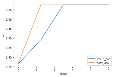
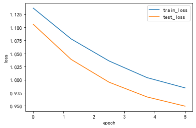
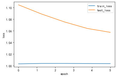
device = torch.device("cuda:0" if torch.cuda.is_available() else "cpu")print("using {} device.".format(device))data_transform = {"train": transforms.Compose([transforms.Resize((64,64)), transforms.RandomHorizontalFlip(), transforms.ToTensor(), transforms.Normalize((0.5,0.5,0.5), (0.5,0.5,0.5))]), "test": transforms.Compose([transforms.Resize((64,64)), transforms.ToTensor(), transforms.Normalize((0.5,0.5,0.5), (0.5,0.5,0.5))])}data_root =os.getcwd()image_path = os.path.join(data_root,"data/vehcileClassificationDataset")print(image_path)train_dataset = datasets.ImageFolder(root=os.path.join(image_path,"train"), transform = data_transform["train"])train_num = len(train_dataset)print(train_num)batch_size = 128train_loader = torch.utils.data.DataLoader(train_dataset, batch_size = batch_size, shuffle = True, num_workers = 0)test_dataset = datasets.ImageFolder(root=os.path.join(image_path,"test"), transform = data_transform["test"])test_num = len(test_dataset)print(test_num)#val_num = 364test_loader = torch.utils.data.DataLoader(test_dataset, batch_size = batch_size, shuffle=False, num_workers = 0)print("using {} images for training, {} images for validation .".format(train_num,test_num))using cuda:0 device./root/autodl-tmp/courses_deep/data/vehcileClassificationDataset1019338using 1019 images for training, 338 images for validation .# 自定义单通道卷积def corr2d(X,K): ''' X:输入,shape (batch_size,H,W) K:卷积核,shape (k_h,k_w) ''' batch_size,H,W = X.shape k_h,k_w = K.shape #初始化结果矩阵 Y = torch.zeros((batch_size,H-k_h+1,W-k_w+1)).to(device) for i in range(Y.shape[1]): for j in range(Y.shape [2]): Y[:,i,j] = (X[:,i:i+k_h,j:j+k_w]* K).sum() return Y#自定义多通道卷积def corr2d_multi_in(X,K): ''' 输入X:维度(batch_size,C_in,H, W) 卷积核K:维度(C_in,k_h,k_w) 输出:维度(batch_size,H_out,W_out) ''' #先计算第一通道 res = corr2d(X[:,0,:,:], K[0,:,:]) for i in range(1, X.shape[1]): #按通道相加 res += corr2d(X[:,i,:,:], K[i,:,:]) return res#自定义多个多通道卷积 def corr2d_multi_in_out(X, K): # X: shape (batch_size,C_in,H,W) # K: shape (C_out,C_in,h,w) # Y: shape(batch_size,C_out,H_out,W_out) return torch.stack([corr2d_multi_in(X, k) for k in K],dim=1) class MyConv2D(nn.Module): def __init__(self,in_channels, out_channels,kernel_size): super(MyConv2D,self).__init__() #初始化卷积层的2个参数:卷积核、偏差 #isinstance判断类型 if isinstance(kernel_size,int): kernel_size = (kernel_size,kernel_size) self.weight = nn.Parameter(torch.randn((out_channels, in_channels) + kernel_size)).to(device) self.bias = nn.Parameter(torch.randn(out_channels,1,1)).to(device) def forward(self,x): #x:输入图片,维度(batch_size,C_in,H,W) return corr2d_multi_in_out(x,self.weight) + self.bias#添加自定义卷积层到模块中 class MyConvModule(nn.Module): def __init__(self): super(MyConvModule,self).__init__() #定义一层卷积层 self.conv = nn.Sequential( MyConv2D(in_channels = 3,out_channels = 32,kernel_size = 3), nn.BatchNorm2d(32), # inplace-选择是否进行覆盖运算 nn.ReLU(inplace=True)) #输出层,将通道数变为分类数量 self.fc = nn.Linear(32,num_classes) def forward(self,x): #图片经过一层卷积,输出维度变为(batch_size,C_out,H,W) out = self.conv(x) #使用平均池化层将图片的大小变为1x1,第二个参数为最后输出的长和宽(这里默认相等了)64-3/1 + 1 =62 out = F.avg_pool2d(out,62) #将张量out从shape batchx32x1x1 变为 batch x32 out = out.squeeze() #输入到全连接层将输出的维度变为3 out = self.fc(out) return outnum_classes = 3 lr = 0.001epochs = 5#初始化模型 net = MyConvModule().to(device) #使用多元交叉熵损失函数 criterion = nn.CrossEntropyLoss() #使用Adam优化器 optimizer = optim.Adam(net.parameters(),lr = lr) def train_epoch(net, data_loader, device): net.train() #指定当前为训练模式 train_batch_num = len(data_loader) #记录共有多少个batch total_1oss = 0 #记录Loss correct = 0 #记录共有多少个样本被正确分类 sample_num = 0 #记录样本总数 #遍历每个batch进行训练 for batch_idx, (data,target) in enumerate (data_loader): t1 = time.time() #将图片放入指定的device中 data = data.to(device).float() #将图片标签放入指定的device中 target = target.to(device).long() #将当前梯度清零 optimizer.zero_grad() #使用模型计算出结果 output = net(data) #计算损失 loss = criterion(output, target.squeeze()) #进行反向传播 loss.backward() optimizer.step() #累加loss total_1oss += loss.item( ) #找出每个样本值最大的idx,即代表预测此图片属于哪个类别 prediction = torch.argmax(output, 1) #统计预测正确的类别数量 correct += (prediction == target).sum().item() #累加当前的样本总数 sample_num += len(prediction) #if batch_idx//5 ==0: t2 = time.time() print("processing:{}/{},消耗时间{}s". format(batch_idx+1,len(data_loader),t2-t1)) #计算平均oss与准确率 loss = total_1oss / train_batch_num acc = correct / sample_num return loss, acc def test_epoch(net, data_loader, device): net.eval() #指定当前模式为测试模式 test_batch_num = len(data_loader) total_loss = 0 correct = 0 sample_num = 0 #指定不进行梯度变化 with torch.no_grad(): for batch_idx, (data, target) in enumerate(data_loader): data = data.to(device).float() target = target.to(device).long() output = net(data) loss = criterion(output, target) total_loss += loss.item( ) prediction = torch.argmax(output, 1) correct += (prediction == target).sum().item() sample_num += len(prediction) loss = total_loss / test_batch_num acc = correct / sample_num return loss,acc#### 存储每一个epoch的loss与acc的变化,便于后面可视化 train_loss_list = [] train_acc_list = [] test_loss_list = [] test_acc_list = [] time_list = [] timestart = time.time() #进行训练 for epoch in range(epochs): #每一个epoch的开始时间 epochstart = time.time() #在训练集上训练 train_loss, train_acc = train_epoch(net,data_loader=train_loader, device=device ) #在测试集上验证 test_loss, test_acc = test_epoch(net,data_loader=test_loader, device=device) #每一个epoch的结束时间 elapsed = (time.time() - epochstart) #保存各个指际 train_loss_list.append(train_loss) train_acc_list.append(train_acc ) test_loss_list.append(test_loss) test_acc_list.append(test_acc) time_list.append(elapsed) print('epoch %d, train_loss %.6f,test_loss %.6f,train_acc %.6f,test_acc %.6f,Time used %.6fs'%(epoch+1, train_loss,test_loss,train_acc,test_acc,elapsed)) #计算总时间 timesum = (time.time() - timestart) print('The total time is %fs',timesum) processing:1/8,消耗时间49.534741163253784sprocessing:2/8,消耗时间53.82337474822998sprocessing:3/8,消耗时间54.79615521430969sprocessing:4/8,消耗时间54.47013306617737sprocessing:5/8,消耗时间54.499276638031006sprocessing:6/8,消耗时间54.50710964202881sprocessing:7/8,消耗时间53.65488290786743sprocessing:8/8,消耗时间53.24664235115051sepoch 1, train_loss 1.136734,test_loss 1.105827,train_acc 0.264966,test_acc 0.266272,Time used 471.139387sprocessing:1/8,消耗时间48.97239923477173sprocessing:2/8,消耗时间52.72454595565796sprocessing:3/8,消耗时间53.08940005302429sprocessing:4/8,消耗时间53.7891743183136sprocessing:5/8,消耗时间53.07097554206848sprocessing:6/8,消耗时间53.59272122383118sprocessing:7/8,消耗时间53.85381197929382sprocessing:8/8,消耗时间54.998770236968994sepoch 2, train_loss 1.077828,test_loss 1.038692,train_acc 0.391560,test_acc 0.573964,Time used 466.846851sprocessing:1/8,消耗时间49.87800121307373sprocessing:2/8,消耗时间50.94171380996704sprocessing:3/8,消耗时间51.578328371047974sprocessing:4/8,消耗时间52.10942506790161sprocessing:5/8,消耗时间53.03168201446533sprocessing:6/8,消耗时间53.60364890098572sprocessing:7/8,消耗时间53.400307416915894sprocessing:8/8,消耗时间53.074254274368286sepoch 3, train_loss 1.035702,test_loss 0.995151,train_acc 0.574092,test_acc 0.573964,Time used 460.014597sprocessing:1/8,消耗时间49.56705284118652sprocessing:2/8,消耗时间50.62346339225769sprocessing:3/8,消耗时间51.27069616317749sprocessing:4/8,消耗时间52.584522008895874sprocessing:5/8,消耗时间53.778876304626465sprocessing:6/8,消耗时间54.50534129142761sprocessing:7/8,消耗时间54.09490990638733sprocessing:8/8,消耗时间53.962727785110474sepoch 4, train_loss 1.003914,test_loss 0.967035,train_acc 0.574092,test_acc 0.573964,Time used 462.696877sprocessing:1/8,消耗时间49.09861469268799sprocessing:2/8,消耗时间50.945659160614014sprocessing:3/8,消耗时间51.85160732269287sprocessing:4/8,消耗时间52.68898820877075sprocessing:5/8,消耗时间52.44323921203613sprocessing:6/8,消耗时间53.98334002494812sprocessing:7/8,消耗时间53.38289451599121sprocessing:8/8,消耗时间53.83491349220276sepoch 5, train_loss 0.984345,test_loss 0.949488,train_acc 0.574092,test_acc 0.573964,Time used 460.776392sThe total time is %fs 2321.475680589676def Draw_Curve(*args,xlabel = "epoch",ylabel = "loss"):# for i in args: x = np.linspace(0,len(i[0]),len(i[0])) plt.plot(x,i[0],label=i[1],linewidth=1.5) plt.xlabel(xlabel) plt.ylabel(ylabel) plt.legend() plt.show()Draw_Curve([train_acc_list,"train_acc"],[test_acc_list,"test_acc"],ylabel = "acc")Draw_Curve([train_loss_list,"train_loss"],[test_loss_list,"test_loss"])
与手写二维卷积除了模型定义和不同外,其他均相同
#pytorch封装卷积层class ConvModule(nn.Module): def __init__(self): super(ConvModule,self).__init__() #定义三层卷积层 self.conv = nn.Sequential( #第一层 nn.Conv2d(in_channels = 3,out_channels = 32, kernel_size = 3 , stride = 1,padding=0), nn.BatchNorm2d(32), # inplace-选择是否进行覆盖运算 nn.ReLU(inplace=True), #第二层 nn.Conv2d(in_channels = 32,out_channels = 64, kernel_size = 3 , stride = 1,padding=0), nn.BatchNorm2d(64), # inplace-选择是否进行覆盖运算 nn.ReLU(inplace=True), #第三层 nn.Conv2d(in_channels = 64,out_channels = 128, kernel_size = 3 , stride = 1,padding=0), nn.BatchNorm2d(128), # inplace-选择是否进行覆盖运算 nn.ReLU(inplace=True) ) #输出层,将通道数变为分类数量 self.fc = nn.Linear(128,num_classes) def forward(self,x): #图片经过三层卷积,输出维度变为(batch_size,C_out,H,W) out = self.conv(x) #使用平均池化层将图片的大小变为1x1,第二个参数为最后输出的长和宽(这里默认相等了)(64-3)/1 + 1 =62 (62-3)/1+1 =60 (60-3)/1+1 =58 out = F.avg_pool2d(out,58) #将张量out从shape batchx128x1x1 变为 batch x128 out = out.squeeze() #输入到全连接层将输出的维度变为3 out = self.fc(out) return out # 更换为ConvModulenet = ConvModule().to(device)#### 存储每一个epoch的loss与acc的变化,便于后面可视化 train_loss_list = [] train_acc_list = [] test_loss_list = [] test_acc_list = [] time_list = [] timestart = time.time() #进行训练 for epoch in range(epochs): #每一个epoch的开始时间 epochstart = time.time() #在训练集上训练 train_loss, train_acc = train_epoch(net,data_loader=train_loader, device=device ) #在测试集上验证 test_loss, test_acc = test_epoch(net,data_loader=test_loader, device=device) #每一个epoch的结束时间 elapsed = (time.time() - epochstart) #保存各个指际 train_loss_list.append(train_loss) train_acc_list.append(train_acc ) test_loss_list.append(test_loss) test_acc_list.append(test_acc) time_list.append(elapsed) print('epoch %d, train_loss %.6f,test_loss %.6f,train_acc %.6f,test_acc %.6f,Time used %.6fs'%(epoch+1, train_loss,test_loss,train_acc,test_acc,elapsed)) #计算总时间 timesum = (time.time() - timestart) print('The total time is %fs',timesum) processing:1/8,消耗时间1.384758710861206sprocessing:2/8,消耗时间0.025571107864379883sprocessing:3/8,消耗时间0.02555680274963379sprocessing:4/8,消耗时间0.025563478469848633sprocessing:5/8,消耗时间0.025562286376953125sprocessing:6/8,消耗时间0.025719642639160156sprocessing:7/8,消耗时间0.025638103485107422sprocessing:8/8,消耗时间0.02569437026977539sepoch 1, train_loss 1.134971,test_loss 1.104183,train_acc 0.131501,test_acc 0.133136,Time used 2.488544sprocessing:1/8,消耗时间0.02553415298461914sprocessing:2/8,消耗时间0.025570392608642578sprocessing:3/8,消耗时间0.025498628616333008sprocessing:4/8,消耗时间0.025622844696044922sprocessing:5/8,消耗时间0.025777101516723633sprocessing:6/8,消耗时间0.0256195068359375sprocessing:7/8,消耗时间0.02576303482055664sprocessing:8/8,消耗时间0.02545619010925293sepoch 2, train_loss 1.134713,test_loss 1.102343,train_acc 0.123651,test_acc 0.239645,Time used 1.160389sprocessing:1/8,消耗时间0.025580883026123047sprocessing:2/8,消耗时间0.025583267211914062sprocessing:3/8,消耗时间0.025578737258911133sprocessing:4/8,消耗时间0.025538921356201172sprocessing:5/8,消耗时间0.025668621063232422sprocessing:6/8,消耗时间0.02561044692993164sprocessing:7/8,消耗时间0.02561807632446289sprocessing:8/8,消耗时间0.02550649642944336sepoch 3, train_loss 1.134326,test_loss 1.105134,train_acc 0.129539,test_acc 0.186391,Time used 1.124050sprocessing:1/8,消耗时间0.025658130645751953sprocessing:2/8,消耗时间0.025626659393310547sprocessing:3/8,消耗时间0.02562260627746582sprocessing:4/8,消耗时间0.02557849884033203sprocessing:5/8,消耗时间0.025677204132080078sprocessing:6/8,消耗时间0.025617122650146484sprocessing:7/8,消耗时间0.02563309669494629sprocessing:8/8,消耗时间0.025460243225097656sepoch 4, train_loss 1.134662,test_loss 1.111777,train_acc 0.127576,test_acc 0.115385,Time used 1.105919sprocessing:1/8,消耗时间0.025597333908081055sprocessing:2/8,消耗时间0.025560379028320312sprocessing:3/8,消耗时间0.025528430938720703sprocessing:4/8,消耗时间0.025620698928833008sprocessing:5/8,消耗时间0.025687694549560547sprocessing:6/8,消耗时间0.025610685348510742sprocessing:7/8,消耗时间0.02558135986328125sprocessing:8/8,消耗时间0.025484323501586914sepoch 5, train_loss 1.134296,test_loss 1.117432,train_acc 0.131501,test_acc 0.106509,Time used 1.103042sThe total time is %fs 6.982609033584595Draw_Curve([train_acc_list,"train_acc"],[test_acc_list,"test_acc"],ylabel = "acc")Draw_Curve([train_loss_list,"train_loss"],[test_loss_list,"test_loss"])
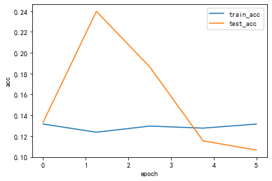
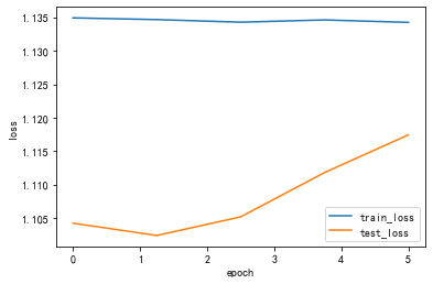
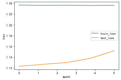
lr_list = [0.1,0.01,0.001]for lr in lr_list : print("lr:",lr) optimizer = optim.Adam(net.parameters(),lr = lr) # 更换为ConvModule net = ConvModule().to(device) #### 存储每一个epoch的loss与acc的变化,便于后面可视化 train_loss_list = [] train_acc_list = [] test_loss_list = [] test_acc_list = [] time_list = [] timestart = time.time() #进行训练 for epoch in range(epochs): #每一个epoch的开始时间 epochstart = time.time() #在训练集上训练 train_loss, train_acc = train_epoch(net,data_loader=train_loader, device=device ) #在测试集上验证 test_loss, test_acc = test_epoch(net,data_loader=test_loader, device=device) #每一个epoch的结束时间 elapsed = (time.time() - epochstart) #保存各个指际 train_loss_list.append(train_loss) train_acc_list.append(train_acc ) test_loss_list.append(test_loss) test_acc_list.append(test_acc) time_list.append(elapsed) print('epoch %d, train_loss %.6f,test_loss %.6f,train_acc %.6f,test_acc %.6f,Time used %.6fs'%(epoch+1, train_loss,test_loss,train_acc,test_acc,elapsed)) Draw_Curve([train_acc_list,"train_acc"],[test_acc_list,"test_acc"],ylabel = "acc") Draw_Curve([train_loss_list,"train_loss"],[test_loss_list,"test_loss"])lr: 0.1processing:1/8,消耗时间0.025880813598632812sprocessing:2/8,消耗时间0.02591729164123535sprocessing:3/8,消耗时间0.025969743728637695sprocessing:4/8,消耗时间0.02597641944885254sprocessing:5/8,消耗时间0.0259091854095459sprocessing:6/8,消耗时间0.025940418243408203sprocessing:7/8,消耗时间0.02597665786743164sprocessing:8/8,消耗时间0.025816917419433594sepoch 1, train_loss 1.236414,test_loss 1.122834,train_acc 0.312071,test_acc 0.266272,Time used 1.150748sprocessing:1/8,消耗时间0.02601909637451172sprocessing:2/8,消耗时间0.026076078414916992sprocessing:3/8,消耗时间0.02595829963684082sprocessing:4/8,消耗时间0.02597641944885254sprocessing:5/8,消耗时间0.025915145874023438sprocessing:6/8,消耗时间0.02601909637451172sprocessing:7/8,消耗时间0.025966167449951172sprocessing:8/8,消耗时间0.025896072387695312sepoch 2, train_loss 1.235889,test_loss 1.126564,train_acc 0.307164,test_acc 0.266272,Time used 1.130118sprocessing:1/8,消耗时间0.025966405868530273sprocessing:2/8,消耗时间0.026023387908935547sprocessing:3/8,消耗时间0.02602076530456543sprocessing:4/8,消耗时间0.025955677032470703sprocessing:5/8,消耗时间0.026730775833129883sprocessing:6/8,消耗时间0.02618265151977539sprocessing:7/8,消耗时间0.025946378707885742sprocessing:8/8,消耗时间0.025950908660888672sepoch 3, train_loss 1.236183,test_loss 1.129753,train_acc 0.311089,test_acc 0.266272,Time used 1.138533sprocessing:1/8,消耗时间0.0259554386138916sprocessing:2/8,消耗时间0.02595067024230957sprocessing:3/8,消耗时间0.025972843170166016sprocessing:4/8,消耗时间0.025902509689331055sprocessing:5/8,消耗时间0.025956392288208008sprocessing:6/8,消耗时间0.02594304084777832sprocessing:7/8,消耗时间0.02598118782043457sprocessing:8/8,消耗时间0.025868892669677734sepoch 4, train_loss 1.235654,test_loss 1.137612,train_acc 0.309127,test_acc 0.263314,Time used 1.147009sprocessing:1/8,消耗时间0.02599787712097168sprocessing:2/8,消耗时间0.025910615921020508sprocessing:3/8,消耗时间0.025928497314453125sprocessing:4/8,消耗时间0.025904178619384766sprocessing:5/8,消耗时间0.025990724563598633sprocessing:6/8,消耗时间0.02588057518005371sprocessing:7/8,消耗时间0.026009321212768555sprocessing:8/8,消耗时间0.02586531639099121sepoch 5, train_loss 1.235978,test_loss 1.151615,train_acc 0.307164,test_acc 0.272189,Time used 1.136342s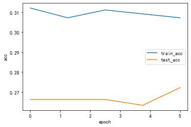
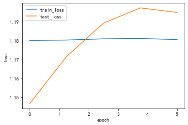
lr: 0.01processing:1/8,消耗时间0.02597332000732422sprocessing:2/8,消耗时间0.025891780853271484sprocessing:3/8,消耗时间0.0260159969329834sprocessing:4/8,消耗时间0.025948286056518555sprocessing:5/8,消耗时间0.026835918426513672sprocessing:6/8,消耗时间0.026047945022583008sprocessing:7/8,消耗时间0.02601790428161621sprocessing:8/8,消耗时间0.0258333683013916sepoch 1, train_loss 1.180047,test_loss 1.146577,train_acc 0.128557,test_acc 0.159763,Time used 1.166165sprocessing:1/8,消耗时间0.025972843170166016sprocessing:2/8,消耗时间0.02600264549255371sprocessing:3/8,消耗时间0.025959253311157227sprocessing:4/8,消耗时间0.025983333587646484sprocessing:5/8,消耗时间0.026042699813842773sprocessing:6/8,消耗时间0.02595233917236328sprocessing:7/8,消耗时间0.025896310806274414sprocessing:8/8,消耗时间0.025844335556030273sepoch 2, train_loss 1.180246,test_loss 1.171511,train_acc 0.134446,test_acc 0.159763,Time used 1.122087sprocessing:1/8,消耗时间0.0258941650390625sprocessing:2/8,消耗时间0.025923728942871094sprocessing:3/8,消耗时间0.02590012550354004sprocessing:4/8,消耗时间0.026006698608398438sprocessing:5/8,消耗时间0.025960922241210938sprocessing:6/8,消耗时间0.02593088150024414sprocessing:7/8,消耗时间0.025939226150512695sprocessing:8/8,消耗时间0.025836944580078125sepoch 3, train_loss 1.180876,test_loss 1.189146,train_acc 0.127576,test_acc 0.159763,Time used 1.112899sprocessing:1/8,消耗时间0.025928497314453125sprocessing:2/8,消耗时间0.025928974151611328sprocessing:3/8,消耗时间0.025905132293701172sprocessing:4/8,消耗时间0.02616095542907715sprocessing:5/8,消耗时间0.02619624137878418sprocessing:6/8,消耗时间0.025908946990966797sprocessing:7/8,消耗时间0.02593541145324707sprocessing:8/8,消耗时间0.025844812393188477sepoch 4, train_loss 1.181045,test_loss 1.197265,train_acc 0.124632,test_acc 0.159763,Time used 1.130010sprocessing:1/8,消耗时间0.025942325592041016sprocessing:2/8,消耗时间0.02595806121826172sprocessing:3/8,消耗时间0.025911331176757812sprocessing:4/8,消耗时间0.026000499725341797sprocessing:5/8,消耗时间0.026007890701293945sprocessing:6/8,消耗时间0.025979042053222656sprocessing:7/8,消耗时间0.02596426010131836sprocessing:8/8,消耗时间0.025872468948364258sepoch 5, train_loss 1.180506,test_loss 1.194845,train_acc 0.130520,test_acc 0.127219,Time used 1.125265s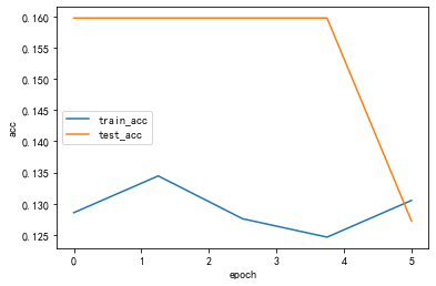
lr: 0.001processing:1/8,消耗时间0.025917768478393555sprocessing:2/8,消耗时间0.02601337432861328sprocessing:3/8,消耗时间0.02601933479309082sprocessing:4/8,消耗时间0.025936603546142578sprocessing:5/8,消耗时间0.025965213775634766sprocessing:6/8,消耗时间0.025942087173461914sprocessing:7/8,消耗时间0.025992393493652344sprocessing:8/8,消耗时间0.025847673416137695sepoch 1, train_loss 1.003024,test_loss 1.104485,train_acc 0.574092,test_acc 0.177515,Time used 1.128456sprocessing:1/8,消耗时间0.025956392288208008sprocessing:2/8,消耗时间0.026005983352661133sprocessing:3/8,消耗时间0.025966167449951172sprocessing:4/8,消耗时间0.0259397029876709sprocessing:5/8,消耗时间0.025922298431396484sprocessing:6/8,消耗时间0.025957107543945312sprocessing:7/8,消耗时间0.02590632438659668sprocessing:8/8,消耗时间0.02581644058227539sepoch 2, train_loss 1.003732,test_loss 1.088773,train_acc 0.574092,test_acc 0.573964,Time used 1.124280sprocessing:1/8,消耗时间0.02595043182373047sprocessing:2/8,消耗时间0.026049375534057617sprocessing:3/8,消耗时间0.02598428726196289sprocessing:4/8,消耗时间0.026129961013793945sprocessing:5/8,消耗时间0.02595376968383789sprocessing:6/8,消耗时间0.02595376968383789sprocessing:7/8,消耗时间0.02597832679748535sprocessing:8/8,消耗时间0.025784730911254883sepoch 3, train_loss 1.003739,test_loss 1.075143,train_acc 0.574092,test_acc 0.573964,Time used 1.123431sprocessing:1/8,消耗时间0.026008129119873047sprocessing:2/8,消耗时间0.0260159969329834sprocessing:3/8,消耗时间0.025996923446655273sprocessing:4/8,消耗时间0.025960683822631836sprocessing:5/8,消耗时间0.02593994140625sprocessing:6/8,消耗时间0.026180744171142578sprocessing:7/8,消耗时间0.025992393493652344sprocessing:8/8,消耗时间0.025855541229248047sepoch 4, train_loss 1.003592,test_loss 1.063867,train_acc 0.574092,test_acc 0.573964,Time used 1.121493sprocessing:1/8,消耗时间0.026531219482421875sprocessing:2/8,消耗时间0.02593708038330078sprocessing:3/8,消耗时间0.0260317325592041sprocessing:4/8,消耗时间0.025905370712280273sprocessing:5/8,消耗时间0.02595996856689453sprocessing:6/8,消耗时间0.026064395904541016sprocessing:7/8,消耗时间0.02595973014831543sprocessing:8/8,消耗时间0.02584242820739746sepoch 5, train_loss 1.003357,test_loss 1.057218,train_acc 0.574092,test_acc 0.573964,Time used 1.131697s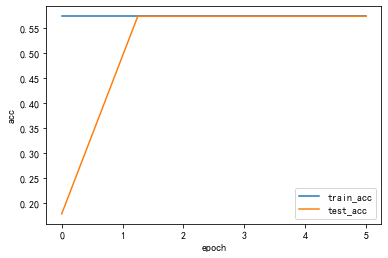
由于输入的图像为64×64,如果按照原始的Alax网络的参数进行定义网络,第一个卷积层的卷积核尺寸为11×11,步长stride为4,导致卷积过后的一些图像尺寸过小,丢失了图像特征,影响模型的精度。因此,本次实验,根据实验数据集的图像特点,对Alexnet网络的特征提取部分参数进行了修改
class AlexNet(nn.Module): def __init__(self,num_classes = 1000,init_weights = False): super(AlexNet,self).__init__() self.features = nn.Sequential(#输入64×64×3 nn.Conv2d(3,48,kernel_size=3,stride=1,padding=1),#64,64,48 nn.ReLU(inplace=True), nn.MaxPool2d(kernel_size=2,stride=2),#32,32,48 nn.Conv2d(48,128,kernel_size=3,padding=1),#32,32,128 nn.ReLU(inplace=True), nn.MaxPool2d(kernel_size=2,stride=2),#16,16,128 nn.Conv2d(128,192,kernel_size=3,padding=1),#16,16,192 nn.ReLU(inplace=True), nn.Conv2d(192,192,kernel_size=3,stride=2,padding=1),#8,8,192 nn.ReLU(inplace=True), nn.Conv2d(192,128,kernel_size=3,padding=1),#8,8,128 nn.ReLU(inplace=True), nn.MaxPool2d(kernel_size=2,stride=2),#4,4,128 ) self.classifier = nn.Sequential( nn.Dropout(p=0.5), nn.Linear(128*4*4,2048), nn.ReLU(inplace=True), nn.Dropout(p=0.5), nn.Linear(2048,2048), nn.ReLU(inplace=True), nn.Linear(2048,num_classes), ) if init_weights: self._initialize_weights() def forward(self,x): x = self.features(x) x = torch.flatten(x,start_dim=1) x = self.classifier(x) return x来源地址:https://blog.csdn.net/mynameisgt/article/details/128279944
--结束END--
本文标题: 深度学习实验3 - 卷积神经网络
本文链接: https://www.lsjlt.com/news/391453.html(转载时请注明来源链接)
有问题或投稿请发送至: 邮箱/279061341@qq.com QQ/279061341
下载Word文档到电脑,方便收藏和打印~
2024-03-01
2024-03-01
2024-03-01
2024-02-29
2024-02-29
2024-02-29
2024-02-29
2024-02-29
2024-02-29
2024-02-29
回答
回答
回答
回答
回答
回答
回答
回答
回答
回答


官方手机版

微信公众号

商务合作


0